Get Indexology® Blog updates via email.

In This List

With VIX Above 80, Expect 5% Daily Swings in the S&P 500

Showtime for Active Managers?

Treasuries Market Flashes Red, Fed Unleashes Tsunami

Liquidity Impacts on Fixed Income ETFs and Passive Investing

Equity Liquidity at a Reasonable Price

With VIX Above 80, Expect 5% Daily Swings in the S&P 500

Contributor Image
Tim Edwards

Managing Director, Index Investment Strategy

S&P Dow Jones Indices

Volatility – it is sometimes said – takes the elevator up but takes the stairs down.  Like seismic activity, volatility can rise precipitously, but tends to decay more slowly; aftershocks and tremors continue to roil markets after any major repricing occurs.  The practical consequence is that, once the markets become volatile, they tend to remain so for some time.  For the short term at least, outsized daily moves will be the new normal.

Exhibit 1: Large Swings Have Become Commonplace

Prior to this month, the last time that the Dow Jones Industrial Average® moved by 5% in a single day was almost 11 years ago.  However, the Dow has swung that much (or more) nearly every day in March, including a single-day decline of 12% on Monday that marked its worst day since the infamous “Black Monday” of 1987.  How long might this continue?

Sometimes called the market’s “fear gauge”, Cboe’s Volatility Index, better known as VIX®, gives an indication of how much volatility the market expects in the near term (or, more accurately, the level of volatility that would justify the current prices of S&P 500® options).  In a history that stretches back over 7,500 trading days to January 1990, five of the eight highest closing levels for VIX occurred in the past week.  Only the peaks in volatility that occurred during the 2008 financial crisis saw anything similar.

Exhibit 2: Five of the highest-ever closes in VIX occurred in the last week.

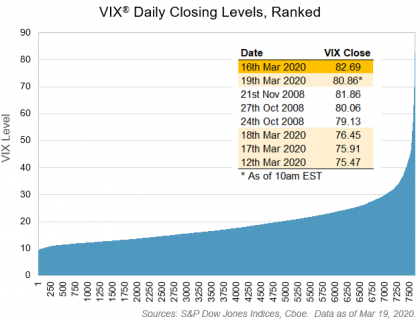
What does a VIX of 80 mean?  In the simplest possible terms, it means that the market expects daily moves in the equity markets to be around four times larger than normal.  Over its long history, the S&P 500 has moved a little under 1% each day, on average.  With VIX currently standing at four times its long-term average of 20, daily moves in the S&P 500 of around 4% are implied for the next month. 

Further, VIX is a forward looking measure, based on traded prices of listed options and with a 30-day horizon for its prediction.  VIX also encodes the expectation that volatility – once elevated – is likely to revert to its average, eventually.  Accordingly, in the very short term, moves of more than 4% should be expected.  Confirming the point, Cboe’s measure of volatility expectations for the next week (the VSXT index) has an index level of 96 (at time of writing), meaning that over the next few trading days, 5% moves in the S&P 500 are the “new normal”.

(For a more in-depth explanation of what information may be usefully discerned from a given VIX level, see our earlier paper, “A Practitioner’s Guide to Reading VIX”)

Beyond the U.S. equity market, indices using the same methodology that VIX uses to reflect S&P 500 volatility expectations have been developed for a range of global indices.  Many of these global volatility indicators are currently indicating similar levels of record-high uncertainty.  Volatility indicators for crude oil and U.S. Treasury bonds made record closing highs yesterday.  Check out the latest readings in S&P DJI’s most recent Risk and Volatility Dashboard.

Further Reading:

The posts on this blog are opinions, not advice. Please read our Disclaimers.

Showtime for Active Managers?

Contributor Image
Anu Ganti

U.S. Head of Index Investment Strategy

S&P Dow Jones Indices

The rapid spread of coronavirus and oil price concerns have whipsawed U.S. equities since the S&P 500® reached its all-time high on Feb. 19, 2020. On March 16, 2020, the index plummeted by 12%, its worst decline since October 1987; as of the close of trading on March 18, 2020, losses for the S&P 500 amounted to 29%. Market commentators have argued that in this environment, active management has an advantage over index funds.

At one level, this argument is correct. We are in precisely the environment in which active portfolio managers have the most potential to add value, since relative returns are easier to achieve when absolute returns are poor.

To understand this, we examine the rise in volatility that has accompanied the stock market’s decline. Higher volatility manifests itself as both higher dispersion and higher correlation; dispersion is a measure of magnitude, while correlation is a measure of timing. We have argued repeatedly that the value of stock-selection skill rises when dispersion is high: a larger gap between winners and losers means that active managers have a better chance of displaying their stock-selection abilities. Exhibit 1 illustrates that dispersion levels in the S&P 500 have jumped since early March 2020.

Higher dispersion also offers greater opportunities for skillful active managers to add value from selecting among sectors, countries, and asset classes. Exhibit 2 shows that dispersion among S&P 500 sectors almost doubled recently, with similar results across countries and asset classes.

Although more nuanced than the obvious advantage of high dispersion, active managers should also prefer high correlations to low correlations. This is because active portfolios are typically more volatile than their index benchmarks; active managers forgo a diversification benefit. When correlations are high, the benefit of diversification falls, as does the benefit forgone, making active management easier to justify.

Exhibit 3 shows that as macroeconomic risk has escalated, correlations have risen; in fact, the reading of 0.8 on March 16, 2020, is an all-time record.

Both high dispersion and high correlations are now working in active managers’ favor. Higher dispersion means that the value of selection skill rises, while higher correlation means that the volatility gap between active portfolios and index funds declines. However, high potential for active value added does not automatically translate into actual value added. Time will tell how active managers will perform in this environment, but at this time next year, when SPIVA® results for 2020 become available—it would not be shocking if active management performance has improved.

The posts on this blog are opinions, not advice. Please read our Disclaimers.

Treasuries Market Flashes Red, Fed Unleashes Tsunami

Contributor Image
Jason Giordano

Director, Fixed Income, Product Management

S&P Dow Jones Indices

As global financial markets grapple with assessing the economic impact of COVID-19, U.S. Treasury yields reached unprecedented levels. On March 9, 2020, the yield on the 10-year U.S. Treasury Bond fell to an intra-day low of 0.32%. This was a drop of more than 125 bps from just three weeks earlier. As market participants fled risk assets, the flight to quality drove the entire U.S. yield curve below 1.00%. The 30-year U.S. Treasury Bond fell to an intra-day low of 0.82% before ending the day at 0.99% (for context, prior to February 2020, the record-low yield in the 30-year Treasury Bond was 1.90% in August 2019). The precipitous fall in yields was staggering, as shown in Exhibit 1.

Perhaps more stunning than the “zero handle” on the 30-year U.S. Treasury Bond was the magnitude and velocity with which the long end of the curve moved. Exhibit 2 shows the rolling weekly volatility of the S&P U.S. Treasury Bond Current 30-Year Index since 2005. As shown, the recent volatility in 30-year U.S. Treasuries far exceeds any previous period, including the Global Financial Crisis, European debt crisis, “Taper Tantrum,” and Brexit referendum.

This historic fall and subsequent rise in yields followed the emergency 50 bps cut the U.S. Federal Reserve implemented on March 3, 2020—only the third occasion in which the Fed cut rates intra-meeting. This action, while clearly necessary, did little to assuage liquidity needs in the market, as Fed Fund futures took less than a week to price in an additional 100 bps cut at the Fed’s March 18 meeting. On March 12, the Fed used its standing repurchase facility to inject an unprecedented amount of liquidity to help meet funding gaps in the short-term market. Exhibit 3 shows the relative size of the increase in offered liquidity in an attempt to help stabilize funding needs.

Less than 72 hours after increasing the repurchase facility to over USD 1 trillion, the FOMC announced yet another emergency intra-meeting rate cut. On Sunday, March 15, the Fed cut rates to a range of 0.00%-0.25%. Exhibit 4 shows the Fed Funds rates since 2015. The first interest rate hike following the Global Financial Crisis occurred on Dec. 15, 2015. It took over four years to get the target range above 2% and less than nine months to go all the way back down to zero.

In a follow-up blog, we will dive deeper into the underlying workings and function of the short-term funding markets. In liquidity events, cracks always show up first in the funding markets and typically ripple through the entire financial system. Exhibits 5 and 6 show the recent spike in option-adjusted spreads (i.e., perceived risk) in the S&P U.S. Dollar Global Investment Grade Corporate Bond Index and the S&P U.S. Dollar Global High Yield Corporate Bond Index.

The posts on this blog are opinions, not advice. Please read our Disclaimers.

Liquidity Impacts on Fixed Income ETFs and Passive Investing

Contributor Image
Brian Luke

Senior Director, Head of Commodities, Real & Digital Assets

S&P Dow Jones Indices

Equity markets have fared reasonably well aided by liquidity in ETFs, as my colleague Craig Lazzara highlights. Steep discounts to net asset values (NAVs) on popular fixed income ETFs are bringing an onslaught of doomsday projections. But while the signs of stress are evident, it’s important to decouple the dysfunction of the bond market from the investment product as well as the manager’s skill.

Let us first consider the market context. The rise of interest rate, credit, and volatility risk was previously discussed as the S&P U.S. Treasury Current 10-Year Index yield fell below 1%. Yields then halved and are now bouncing between 0.5% and 1%. Treasury bid-ask spreads were reported to widen to beyond 1 point and NAV discounts were seen in treasury and credit ETFs. Despite that illiquidity, fixed income ETFs experienced their largest daily volume in treasury and credit sectors. Liquidity is a premium. The Cboe/CBOT 10-year U.S. Treasury Note Volatility Index hit its highest point since the end of Lehman Brothers. This measure, along with its credit and swap variants, highlights the stress experienced across the fixed income markets.[1]

In terms of measuring the impact of these shocks on ETFs, Andrew Upward at Jane Street produced a great historical summary that was covered in a recent S&P Global webinar. In times of credit stress, the discount as a percentage of NAV reflects the price buyers are willing to pay.  In recent days, the largest investment-grade and high-yield ETFs traded at over a 5% discount. This could be misinterpreted as a sign a credit ETF isn’t functioning well. There are a few critical points to counter that view. First, prices in the over-the-counter bond market are typically shown as “request for quote”—as soon as one wishes to sell at an advertised price, the trader showing the bid can remove it. The fact that an ETF has an executable price goes well beyond the unwilling participants in the OTC market. The second critical point is the latency in NAV calculation. As an index provider, we pride ourselves on using independent transparent pricing.  These price providers play a heavy role in NAV calculation and are often referred to as price “evaluators,” since they are providing their evaluation on what the price of a bond should be on a given day. Having an independent resource is critical for the index and fund administration community. But they are not employing exacting measures to determine the price of a bond that may or may not have traded that day. The last point is a timing issue; the official index closes at 3PM, while the ETF and its NAV close at 4:00PM.  This also causes a mismatch to NAV during times of volatility.

In the webinar, Bill Ahmuty, Head of SPDR Fixed Income Group at State Street Global Advisors, spoke about how fixed income volumes tend to grow during times of stress, while the underlying cash bond market volume tends to shrink. It appears that ETFs fulfill a critical need of liquidity when liquidity is needed most. ETF structure lends well to this, as investors can trade ETF shares without having to source the individual bonds. This only works to the extent that buyers and sellers can match their trades. Once they are matched, the liquidity must be met by the underlying bond market. As the fixed income ETF market grows, it has a better opportunity to meet or improve liquidity, similar to the equity market.

Finally, as investors look for those who successfully navigated these markets, the active versus passive debate will return. While that argument may be over for equity, new index-based strategies are proving their worth in fixed income. We will cover passive strategies and their performance in upcoming posts, but now, we want to highlight how the S&P U.S. High Yield Low Volatility Corporate Bond Index has outperformed its benchmark by 2.4% YTD.

While fixed income ETFs have largely performed in line with this market, the growth of secondary market trading will continue to help face future liquidity needs.

[1] For more information on this topic, please see the S&P Global webinar Measuring Fixed Income Volatility.

The posts on this blog are opinions, not advice. Please read our Disclaimers.

Equity Liquidity at a Reasonable Price

Contributor Image
Craig Lazzara

Former Managing Director, Index Investment Strategy

S&P Dow Jones Indices

The fall in equity market values since February’s peak has been sudden and dramatic.  During this period, the equity markets have functioned well at their primary task of facilitating price discovery at a time when values were changing rapidly.  Equity investors who wanted to trade have been able to trade.  (Whether they were wise to do so is a separate question.)

This is in no small part due to the liquidity provided by index-linked vehicles.  Index funds have been part of the investment landscape for nearly 50 years, during which time superior performance and low cost have earned them a growing share of investor assets.  What’s less well-appreciated has been the growth of a trading ecosystem linked to indices, most importantly to the S&P 500.  The vast majority of trading in index-linked vehicles is not done by index funds, but rather by active investors and traders.

The coronavirus-induced bear market which we’re now enduring illustrates the logic of index-linked trading well.  A pandemic of still-unknown duration and severity can be expected to affect every business adversely.  The degree of adversity will obviously vary across industries, with some (e.g., airlines and hotels) suffering more than others.  But investors who want to adjust equity exposures quickly will be far better served by trading an entire index than by trying to sort out relative winners and losers in the traditional way.

In this environment, it’s unsurprising to see higher volumes and higher dealer spreads, as we did during the last two weeks’ market carnage.  It’s estimated that in the first week of March, “exchange-traded products powered more than a third of equities trading on U.S. exchanges.”  We can see this effect in Exhibit 1, which measures the average value traded in the largest ETF tracking the S&P 500.  Normally the most heavily-traded issue in the U.S. market, daily volume skyrocketed at the end of February.

Exhibit 1. Trading Volume Spiked During the Market Decline

Source: S&P Dow Jones Indices, Bloomberg. Data from Jan. 3, 2012 to March 16, 2020. Graph is provided for illustrative purposes.

At the same time trading costs rose, as measured by the width of the bid-offer spread pictured in Exhibit 2.

Exhibit 2.  Spreads Widened

Source: S&P Dow Jones Indices, Bloomberg. Data from Jan. 3, 2012 to March 16, 2020. Graph is provided for illustrative purposes.

As recently as January 2020, spreads were as low as 0.003%; more recently they doubled.  Spreads are not at all-time highs, however, and trading the ETF is still much cheaper than trading individual securities.

It’s important to understand that the widening of dealer spreads is a natural and appropriate reaction to the extraordinary levels of market volatility we’ve witnessed since mid-February.  Exhibit 3 describes the relationship between the VIX index and the ETF’s bid-asked spread.  When VIX is at or below its median level, for example, spreads average just over $0.01/share.  The relationship slopes gently upward over most values of VIX.  Extreme levels of VIX, however, indicate heightened dealer risk, and thus increased bid-asked spreads.

Exhibit 3.  Higher VIX Leads to Wider Spreads

Source: S&P Dow Jones Indices, Bloomberg. Data from Jan. 3, 2012 to March 16, 2020. Graph is provided for illustrative purposes.

At time when it was badly needed, index-based products helped to ensure equity liquidity was available at a reasonable price.

The posts on this blog are opinions, not advice. Please read our Disclaimers.