Indexology^® Blog

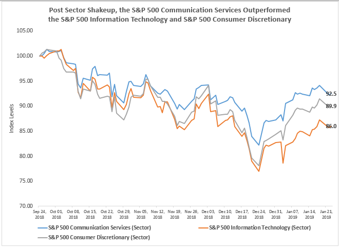
Since the sector shakeup on Sep. 24, 2018,  the S&P 500 fell 19.5% through the close of Dec. 24, 2018 then rebounded 12.2% by the close of  Jan. 23, 2019 for a loss of 9.6% in the full period.  The annualized volatility of 22.8% in the past 82 days has been the highest since the 82 days ending Feb. 1, 2012, when the level was 22.9%.  While the volatility is higher than the 15.7% average for 82-day periods since Jan. 4, 1928, it is not near the high of 65.5% that occurred in the 82-day period ending on Jan. 2, 2009.  Nonetheless, the distinct down and up periods are interesting to evaluate, especially for the newly configured sectors.

Inside of the S&P 500 on Sep. 24, 2018, the market capitalization ($MM) for communication services was 2,444,289, consumer discretionary was 2,501,033 and information technology was 5,133,491, which resulted in respective index weights of 9.9%, 10.2% and 20.8%.  This meant information technology was the biggest sector in the S&P 500, consumer discretionary was the fourth largest and and communications services was the fifth largest.  Through Dec. 24, 2018, the S&P 500 Information Technology lost 23.1%, the S&P 500 Consumer Discretionary lost 22.0% and the S&P 500 Communication Services lost 17.8%.  Of the three sectors, only the communication services sector avoided a bear market and outperformed the S&P 500.

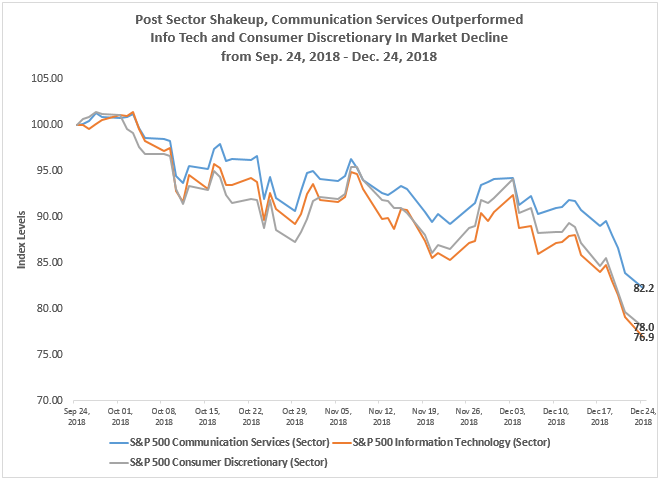
The losses were severe in all three sectors, with market capitalization ($MM) declines of 437,154, 565,886 and 1,196,100 in communication services, consumer discretionary and information technology, respectively.  However, since the communication services sector held up better than the consumer discretionary sector, its index weight gained 0.25% while the index weight of consumer discretionary lost 0.35%.  This propelled communication services to become the fourth largest sector, weighing 10.2% of the S&P 500, overtaking consumer discretionary, which fell to the fifth spot, with an index weight of 9.8%.  The information technology sector remained the largest though its weight dropped to 20.0%.

Despite better performance of 15.3% from the consumer discretionary sector than of 12.5% from communication services from Dec. 24, 2018 through Jan. 23, 2018, when the S&P 500 gained 12.2%, the communication services has held its place as the fourth largest sector.  In this time-frame, communication services gained 250,482 of market capitalization ($MM), slightly less than the 295,316 gained in consumer discretionary, resulting in an increasing index weight of 10.1% in consumer discretionary versus a nearly constant 10.2% in communication services.  Through the period, information technology, though recovering 459,319 of its market capitalization ($MM), lost a full percentage point of its weight since the sector shuffle, now with an index weight of 19.8%, but still the largest.

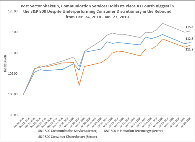
While the rebound has not been big enough to recoup all the losses in these sectors, overall the communication services held up best from Sep. 24, 2018 – Jan. 23, 2019.  Over the period, the S&P 500 Communication Services lost 7.5% as compared to the S&P 500 Information Technology that lost 14.0% and the  S&P 500 Consumer Discretionary that lost 10.1%.

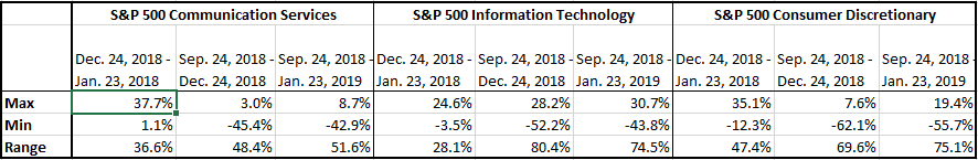
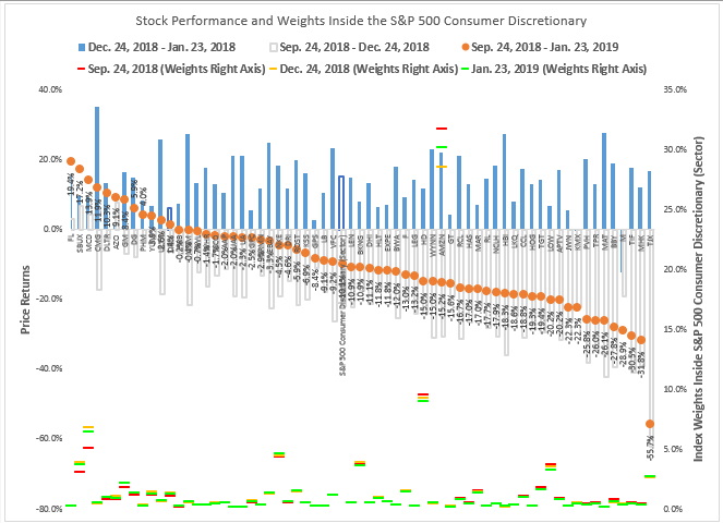
Though the stocks within each sector performed differently, most of them moved in the same direction from these overarching pressures.  The range of stock performance was tightest inside the communication services sector with a range of 51.6% between the best performer, TRIP, up 8.7%, and worst performer ATVI, down 42.9% over the period.  Both information technology and consumer discretionary had a spread of 75% between the best and worst performers.

Source: S&P Dow Jones Indices.

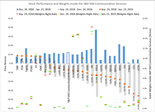
In the S&P 500 Communication Services, 7 of the 26 stocks in the sector gained over the full period measured: TRIP 8.7%, FOX 8.5%, TWTR 8.3%, FOXA 8.1%, VZ 7.9%, OMC 7.3% and CMCSA 3.5%.  All 26 stocks gained in the rebound period, while TRIP, FOX and FOXA gained a respective 3.0%, 0.9% and 0.9% also in the declining period. VZ overtook T in weight, rising from 9.1% to 10.6% of the sector, now only smaller than GOOG/GOOGL and FB.

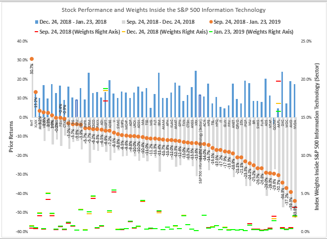
In the S&P 500 Information Technology, only 6 of the 65 stocks in the sector gained over the full period measured: RHT 30.7%, XLNX 13.2%, AVGO 3.2%, VRSN 2.6%, INTC 2.2% and PYPL 1.0%.
Every stock gained in the rebound period except QCOM, which lost 3.5%, while RHT and XLNX gained a respective 28.2% and 0.2% during the declining period. MSFT overtook AAPL in weight, rising from 17.1% to 18.8% of the sector, while AAPL diminished from 19.7% to 15.8% of the sector.

Lastly, in the S&P 500 Consumer Discretionary, 12 of the 64 stocks in the sector gained over the full period measured: FL 19.4%, SBUX 17.2%, MCD 13.9%, CMG 11.9%, DLTR 10.3%, AZO 9.1%, GM 8.4%, DG 5.9%, PHM 4.0%, YUM 3.9%, ULTA 2.6% and ORLY 1.4%.   Every stock gained in the rebound period except M and KMX, which lost 12.3% and 0.1%, respectively.  In the declining period, AZO, SBUX, MCD and FL held up, gaining a respective 7.6%, 6.8%, 4.3% and 3.1%.  AMZN fell in weight from 31.7% to 30.2% of the sector and remains dominant with HD as the next biggest stock, comprising 9.0% of the sector.

It is important to remember the GICS (Global Industry Classification Standard) aims to reflect the market landscape, and why the sector changes happened.  Sector fundamentals are important in driving performance of stocks that are classified together, especially in sub-industry groups.  However, sometimes there are more influential, overarching forces, as we may be experiencing now like the Fed, Brexit and the trading tensions that are responsible for the broad-based moves.

The fourth quarter of 2018 was pretty turbulent for global equities.  Volatility and correlations rose, the majority of the S&P Global BMI’s 48 country constituents declined by double digits, recent darlings among factor strategies (momentum and growth) lagged, and the S&P 500’s 13.52% quarterly plunge left the benchmark with its first calendar-year loss in a decade.  Navigating the heightened volatility environment was likely a priority for many market participants.

Exhibit 1: Most country constituents of the S&P Global BMI declined by double digits in Q4Source: S&P Dow Jones Indices’ “Daily Dashboard”.  Data as of Dec. 31, 2018.  Returns calculated in USD.  Past performance is no guarantee of future results.  Chart is provided for illustrative purposes only.

Perhaps unsurprisingly, more defensive equity strategies typically receive greater attention during periods of heightened volatility.  Against that backdrop, we review stylized examples of asset allocation strategies using the S&P 500, the S&P 500 Low Volatility Index, and the S&P U.S. Treasury Bond Index.

Exhibit 2 shows the impact of switching S&P 500/S&P U.S. Treasury Bond allocations from 70%/30% to 50%/50% each month, depending on whether the S&P 500’s subsequent monthly total return was positive or negative, respectively.  These allocations were chosen so that, on average over the entire period, the hypothetical asset allocation strategy allocated 60% to equities and 40% to bonds.  Armed with a prediction that correctly identified the directional movement in the S&P 500 over the next month with 52% accuracy, the hypothetical “asset allocation” strategy could have provided higher risk-adjusted returns than a hypothetical 60% equity and 40% fixed income allocation, rebalanced monthly.

Exhibit 2: Asset allocation offered higher risk-adjusted returns compared to a static portfolio.

Given there is no crystal ball that tells us whether the S&P 500 will rise or fall over the next month, an asset allocation strategy runs the risk of not obtaining the desired downside protection, or missing out on equity market gains, if predicted outcomes do not materialize.  One way to bypass this issue is to maintain static equity and fixed income allocations, and to incorporate equity factor strategies designed to mitigate downside risks.  Low volatility may be an appealing choice for many, given its historical propensity to marry downside protection and upside participation.

Exhibit 3 shows the cumulative total returns of a hypothetical “low vol equity” portfolio with static 30%/30%/40% allocations to the S&P 500/S&P 500 Low Volatility/S&P U.S. Treasury Bond Index, rebalanced monthly.  The hypothetical portfolio offered greater downside protection than either of the 60/40 or asset allocation strategies: on average, the low vol equity portfolio captured 44.8% of S&P 500 returns during months when the equity benchmark declined, compared to over 50% for the other hypothetical portfolios. This helped it to outperform on a risk-adjusted basis, historically.

Exhibit 3: The hypothetical “low vol equity” strategy outperformed on a risk-adjusted basis.

Of course, there are many ways that market participants may seek to navigate equity market turbulence and there are many different paths that returns could take when using an uncertain prediction.  But the above example shows how incorporating low volatility within a static equity allocation could act as an alternative to adjusting asset allocations.  Not only would such a strategy bypass the difficulty in correctly timing the market, but it could have improved upon the hypothetical performance of an asset allocation strategy, historically.

2018 produced negative absolute returns across a number of asset classes, particularly international stocks. A broad benchmark of stocks traded outside of the U.S., the S&P Global ex-U.S. BMI (US Dollar) Gross Total Return Index, lost 14.18% of its value. Nevertheless, many investments kept pace with the change in cost of securing future retirement income, because an upward shift of real rates decreased the present value of future inflation-adjusted cash flows. For instance, the constant maturity 10-Year Treasury Inflation-Indexed Security Rate,[1] published by the St. Louis Fed, almost doubled from 0.54% in January 2017 to 1.02% on Dec. 1, 2018.

Exhibit 1 shows the change in present value, for 2017 and 2018, of 25-year inflation-adjusted cash flows that begin paying in the respective future years on the chart’s horizontal axis. For example, savers planning to retire around 2030 saw the cost of providing themselves 25 years of inflation-adjusted income decrease by 9.96% in 2018 after an increase of 7.51% in 2017.

Exhibit 2 shows the total returns of U.S. stocks and bonds, as measured by the S&P 500^® and the S&P U.S. Aggregate Bond Index, as well as a hypothetical 60/40 mix of the two, for 2017 and 2018.

Exhibit 3 displays excess total returns of the benchmarks from Exhibit 2 over the decrease in the cost of income for each respective year (from 2020 to 2060). Despite negative and near-zero absolute returns for U.S. stocks and bonds, respectively, both outpaced the change in cost of future income for all of the target years, as did the 60/40 stocks/bonds mix.

Finally, Exhibit 4 shows excess returns of specific S&P STRIDE Indices over the decrease in cost of future income for the same target years.

The S&P STRIDE Indices also outpaced the decrease in cost of future income for all target years from 2020 to 2060. The magnitude of their excess returns over the decrease of income cost was generally not as strong as it was for U.S. stocks and bonds. However, these indices are designed to adjust to changes of income cost more reliably than stocks or bonds. One of the characteristics of the S&P STRIDE Index Series methodology[2] is that the index weight of near-dated S&P STRIDE Indices is heavily allocated to a mix of U.S. Treasury Inflation-Protected Securities matching the duration of retirement income for the respective target year.

If income risk is not managed, the question of whether investment returns will keep pace with changes in income cost is unpredictable, because the relationship between the value of assets and the value of a retirement income liability is essentially random. 2018 provided an example of negative absolute returns outpacing a decrease in the cost of income, so investors saving for retirement may not be as bad off as they feel when they open their year-end 401(k) statements. It may not be immediately apparent, but in income terms, the 2018 scenario is better than a situation wherein positive absolute returns fail to keep pace with increases of income cost. In such a scenario, investors may feel wealthier without considering that their wealth buys less income. Of course, the most detrimental scenario is when negative absolute returns combine with rising income cost, in which case one loses ground in terms of both wealth and income, which may be the strongest argument for managing income risk as retirement draws closer.

[1]   See https://fred.stlouisfed.org/series/FII10.

[2]   https://spindices.com/documents/methodologies/methodology-sp-stride-index-series.pdf

It is that time of year when we look back at the memorable moments that made 2018 so special. In our case, we will look at the Latin American markets to see their development and performance. This past year was particularly exhilarating and terrifying at the same time, similar to the feeling one gets when riding a rollercoaster. The ups and downs make you sick, you scream for help, you want to get off—but once you’re on it, there is nothing you can do but ride the monster. After it is all over and despite the aggravation and fear, you cannot wait to get back on it. Welcome to the Latin American rollercoaster.

The last quarter of 2018 was particularly horrifying for most global markets, with the S&P 500^® giving back nearly 14%. The S&P Europe 350^® and the S&P/TOPIX 150, which seeks to measure Japanese blue chip companies, lost 13% and 15%, respectively. This resulted in global returns of nearly -13% for the quarter, as reflected by the S&P Global 1200, which is designed to measure the 1,200 most important stocks in the world.

Despite the gloom and doom of the fourth quarter, Latin America actually did well compared with other regions. The S&P Latin America BMI, which measures companies in Brazil, Chile, Colombia, Mexico, and Peru, had a positive return of 1.2% in U.S. dollars, while the widely used S&P Latin America 40 was flat at -0.1%. Over the entire year, the S&P Latin America 40, which returned -6%, did not fare as well as the S&P 500, which yielded -4%. However, it did well compared with the S&P Europe 350 and S&P/TOPIX 150, which had returns of -14% and -13% for the year, respectively.

What fueled the Latin American rollercoaster of 2018? The region underwent some of the most important changes it had seen in many years. In 2018, there were major presidential elections in Brazil, Colombia, and Mexico, and new presidents took office in Chile (following the 2017 elections) and Peru (following the resignation of the recently elected president). Chile and Colombia elected moderate candidates, while Brazil and Mexico chose different administrations from the ones that had governed those countries previously. The potential changes brought great uncertainty to the region and, with it, great volatility to the markets.

While most countries ended in the red for the quarter, Brazil was the shining star of the region, with the S&P Brazil BMI returning nearly 15% in U.S. dollars—no other country in Latin America came anywhere near this return. In U.S. dollar terms, Mexico and Colombia had the worst returns. The S&P/BMV IPC was down nearly 20%, and the S&P Colombia Select Index was down almost 18%. While Chile and Peru also had negative returns for the quarter, their returns did not drop as much as the two other countries. The S&P Chile LargeMidCap, a proxy for the S&P/CLX IPSA, returned -3.4% in U.S. dollars, and the S&P/BVL Peru Select Index posted -2%. In their respective local currencies, the indices had better performance.

Looking at longer periods, local investors from Argentina fared the best. Peruvian and Brazilian investors were somewhat behind but still held on to significant returns. Argentina generated returns of over 51% and 48% for the three- and five-year periods, respectively. However, the large devaluation of the Argentine peso against the U.S. dollar and the high inflation rates diminish the value of the returns. Following Brazil’s election of a “market-friendly” presidential candidate, the country entered into a rally that sustained the gains of the three- and five-year periods. The S&P Brazil BMI showed U.S. dollar returns of 27% and 11%, respectively. Peruvian investors also managed to hold on to their gains for these periods, with the S&P/BVL Peru Select Index reporting 27% and 8% in local currency, respectively. Chile did well for both periods, while Colombia had mixed results, with a positive return for the three-year period but a nearly flat local currency return for the five-year period.

In 2018, Mexico struggled to hang on to past gains. The uncertainties of the new government’s policies, the renegotiation of the North American Free Trade Agreement (NAFTA), and the fall of the Mexican peso brought uncertainty and volatility. The market is still struggling to find its footing, although during the first two weeks of 2019 (Jan. 1-14, 2019), the S&P/BMV IPC displayed a positive upturn of nearly 5%.

This new year has so much to look forward to. Latin American is poised for great changes with all these new leaders. It will be interesting to see the direction they take their countries and the outcomes and opportunities this will bring to local and international investors.

To see more details about performance in Latin America, please see: S&P Latin America Equity Indices Quantitative Analysis Q4 2018.

Despite a rocky start and end to 2018 that negatively affected the performance of all the asset classes within the S&P MARC 5% Excess Return (ER) Index,[1] the index maintained a relatively stable performance throughout the year, although it ended the year in red. When you look at the asset classes in the S&P MARC 5% ER, on an excess return basis, equities, as measured by the S&P 500^®, and commodities, as measured by the S&P GSCI Gold, had the largest losses with -6.1% and -4.7%, respectively (see Exhibit 1). Taking these returns and multiplying them by the average weight of the asset classes in the index provides a good indication of which asset classes affected the index performance the most.

What is surprising is that 2018 started on different footing from where it ended. Looking at early 2018, with the exception of February to April, there was a clear dispersion of performance between the different underlying asset classes, and that became more pronounced after April when equities began to rally and gold sold off through the end of Q3 2018. Looking at Q4 2018, the bifurcation of performance continued with equities selling off sharply, while the other asset classes and the S&P MARC 5% ER moved higher toward the end of the year.

When comparing the component assets to the S&P MARC 5% ER to see what periods the components outperformed or underperformed the index, the story is similar. The diversification built into the index design shows that no single asset class consistently performed in line with the S&P MARC 5% ER throughout 2018, but that instead there was a diversification of relative performance between the components and the index itself (see Exhibit 3).

On the surface, it looks like the index was allocated to cash after the February drawdown because of the almost sideways performance; however, when looking at the index weights, what becomes apparent is the index allocation throughout the year. Unlike many other strategy indices, which moved to cash or short-dated Treasuries for extended portions of 2018, the S&P MARC 5% ER held sizeable positions across equities, Treasuries, and gold with an average of 23%, 84%, and 28%, respectively. In addition to the distribution across asset classes, the S&P MARC 5% ER had an average index allocation of 135.7% in 2018.

For more information, please see the S&P MARC 5% Index Methodology.

[1]   Throughout the rest of this blog, the S&P MARC 5% Excess Return Index will be referred to as the S&P MARC 5% ER.