Get Indexology® Blog updates via email.

In This List

The Much-Maligned Market Portfolio

Commodities Ex-Energy Are Fine Despite Contango

The Growth of Small Caps in India

Rieger Report: Munis - "The Kids are Alright"

Inflation, Rising Rates Can Spark Oil's Rebound

The Much-Maligned Market Portfolio

Contributor Image
Philip Murphy

Former Managing Director, Global Head of Index Governance

S&P Dow Jones Indices

It seems generally acknowledged that no investment strategy should be expected to offer an optimal trade-off between return and risk in all periods.  Yet I often hear criticism of market-cap weighting, presumably because modern portfolio theory (MPT) postulates a hypothetical market portfolio as efficient in the mean-variance sense.  Financial engineers, product developers, and asset managers point to a growing range of alternatively weighted strategies designed to capture various risk premia or market anomalies.  In other words, they seek to harvest greater mean-variance efficiency than cap weighting.  While we all want more return per unit of risk, it is nevertheless worth remembering a few salient characteristics and benefits of cap weighting.

First off, all non-market-cap-weighted strategies aggregate into the market portfolio, which by definition is a cap-weighted portfolio.  Therefore, cap-weighting is the only approach that provides a model of the market.  If one seeks equity returns but has no basis upon which to develop security or factor-level return expectations, buying a model of the market avoids guesswork.

Secondly, market-cap weighting is transactionally efficient and tax efficient, requiring only minimal rebalancing to account for changes in shares outstanding.  I have heard it stated that as companies become larger, there is forced buying of their shares in index funds, but that is not the case.  When a company’s market cap grows, existing shareholders only need to continue holding their shares.  Only net new cash flows into index-based funds (or active funds) produce buying to the extent that asset managers wish to avoid cash drag.  There are also highly liquid exchange-traded derivatives that, in addition to cash market share purchases, offer efficient means of cash equitization.

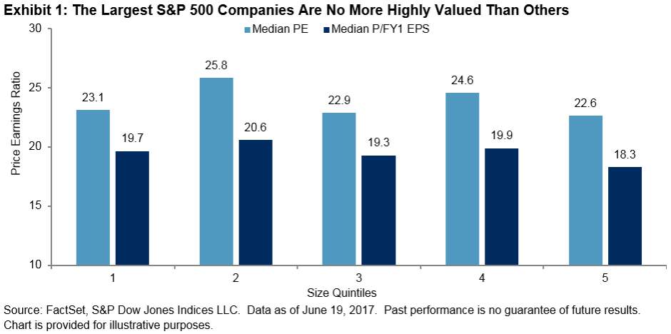
Lastly, and perhaps related to the forced buying theory above, market-cap weighting is criticized for promoting overvaluation and enabling stock price bubbles.  The premise here seems to be that the largest stocks are the most expensive.  There may be historical examples of such conditions, like the bubble in information technology shares in the late 1990s, but these periods are much more the exception than the rule.  As of mid-June 2017, the largest companies in the S&P 500 (those making up Quintile 1 in Exhibit 1) were no more highly valued relative to past earnings—or expected future earnings—than others.

Factors such as value, momentum, and quality, as well as other alternatively weighted investment approaches, may offer enhanced mean-variance efficiency in particular periods, but it is a Herculean task to identify risk premium leadership period to period and year to year.  Many investors would be better off in the long run choosing a model of the market, trying to save more, and identifying an appropriate level of overall equity exposure that considers their circumstances and risk tolerance.  It’s all about blocking and tackling for a lifetime.

The posts on this blog are opinions, not advice. Please read our Disclaimers.

Commodities Ex-Energy Are Fine Despite Contango

Contributor Image
Jodie Gunzberg

Former Managing Director, Head of U.S. Equities

S&P Dow Jones Indices

Energy is back in a bear market now led by oil’s slide mainly due to rising output from Libya and Nigeria, two OPEC members exempt from cutting supply.  The S&P GSCI Energy Total Return is on pace for its worst quarter since the fourth quarter of 2015 losing -13.4% quarter-to-date (through June 19, 2017.) This is driven by the Brent crude and (WTI) crude oil in the index that are also having their worst total returns since Q4 2015, losing 13.7% and 13.9%, respectively.  In turn the S&P GSCI Total Return is also suffering with a loss of -8.3% in the quarter thus far, on pace to be its worst quarter since Q4 2015.  However, ex-energy, commodities are doing fine.

Source: S&P Dow Jones Indices. Data ending June 19, 2017.

Though energy’s impact on the broad commodity index is weighing the S&P GSCI Total Return down 12.9% year-to-date, investors are highly interested as commodities have rebounded more than 13% off their bottom on Jan. 20, 2016. Also, ex-energy commodities are up slightly this year with some like wheat (+8.6%,) cattle(+15%,) aluminum (+10.3%) and gold (+7.7%) up substantially.  Now many investors fear political risk, weakness in the financial sector and uncertainty about global economic growth, so turn to gold as a safe haven.  Others seem to like trading around the volatility in oil despite the drop, and the rest of the demand is mainly from the chance to enter the asset class at attractive levels for the longer-term benefits of inflation protection and diversification.

With the renewed interest in commodities as an asset class has also come more concern about contango, a term-structure condition where futures contracts with nearby expiration dates are cheaper than contracts with later-dated expiration dates.  The result of contango is a roll return loss from selling the cheaper, expiring contracts to buy more expensive later-dated ones.  (There is also an opposite condition called backwardation that is profitable to investors.)  Contango happens when there are high storage costs from excess inventories, which has been the case as commodities have been substantially oversupplied.

Since commodities have been in contango since Aug. 2015 as measured by the roll yield (excess return – spot return of the S&P GSCI,) many investor think commodities are always in contango.  However, this is certainly not the case, so below are some charts to demonstrate exactly how much time commodities spend in each condition of backwardation and contango.  The black lines represent months in backwardation and the white lines represent months in contango.  Overall, the commodities have spent about 60% of months in contango and 40% in backwardation.  On average the roll return gain from backwardation is 1.1% in a month and the roll loss from contango is -0.9% from contango in a month, yielding a weighted average of about -0.1% in a month over time.

Source: S&P Dow Jones Indices

Unleaded gasoline spends 57% of months in backwardation, the most time of all the commodities. On the other hand, aluminum spends just 10% of its months in backwardation, the least of all the commodities.  On average in a month, the roll return gain from unleaded gasoline is 20 basis points and the loss from aluminum is about 50 basis points.  Note the difference in the pattern of the two term structure charts.

Source: S&P Dow Jones Indices


Most metals (except copper) are oversupplied like aluminum but the pattern of inventory is different.  For example gold is almost always in contango, about 80% of months, loses only about 40 basis points on average since it is relatively cheap and easy to store.  Zinc is almost 90% in contango and loses about the same on average as gold, but again, notice the inventory pattern is quite different with the big block of backwardation shown in black from a shortage. On the other hand, copper is much less oversupplied and is difficult to store so has a more persistent term structure commanding higher premiums, gaining 0.9% on average in backwardated months versus losses of 0.6% during months in contango to average a total monthly gain of 0.1%.

Source: S&P Dow Jones Indices

For perishable commodities in agriculture like sugar and corn, notice how frequently their term structures change as suppliers try to adjust though weather can interfere with decisions.  The inventories are also relatively difficult to store so, the weighted loss on average is -0.7% for corn and -0.5% for sugar.

Source: S&P Dow Jones Indices

Lastly, the most popular commodities, Brent crude and (WTI) Crude oil that are so oversupplied right now, are not always in contango, although they have been in the condition since July (for Brent) and Dec. (for WTI) 2014. For Brent, the 35 months is a new record, following its longest prior streak of 32 months ending in Dec. 2010.  However, (WTI) Crude oil now in its 30th consecutive month in contango has had one longer bout of contango that lasted 36 months ending Oct. 2011.  While they are concurrently in contango, they are not always moving together and the premiums from WTI are greater.  On average WTI gains 1.7% in a month in contango while losing 1.5% during a backwardated month, though Brent loses 1.1% versus a gain of just 0.9%.  These differences drive one of the most popular spread trades and continue to present opportunities that the market has been interested in to trade the volatility.

Source: S&P Dow Jones Indices

Please click on the link here to read about how long the oil contango might last, and to see more detail about the history of backwardation and contango per commodity, please reference the table below.

Source: S&P Dow Jones Indices


The posts on this blog are opinions, not advice. Please read our Disclaimers.

The Growth of Small Caps in India

Contributor Image
Ved Malla

Associate Director, Client Coverage

S&P Dow Jones Indices

Over the past few decades, Indian capital markets have matured, and a large number of Indian market participants are now looking at capital markets as an investment avenue.  Investment in capital markets has grown substantially among all types of market participants—retail, institutional, and even government institutions, where recently the Employee Provident Fund Organization has started to invest in capital markets via exchange-traded funds.

Traditionally, the tendency of market participants has been to buy large-cap, blue-chip companies that form part of large-cap indices like the S&P BSE SENSEX.  However, there has been a paradigm shift in investment patterns—market participants are now going beyond traditional large-cap companies and venturing into companies in the mid-cap and small-cap segments.  This changing investment pattern has been reflected in equity volumes and performance of stocks in these segments.

Small-cap stocks outperformed large-cap stocks by significant margins in the three-year period ending May 31, 2017.  This significant outperformance by small-cap stocks has resulted in more market participants looking at the small-cap segment.

The S&P BSE Indices include two indices in the small-cap space—the S&P BSE SmallCap and the S&P BSE SmallCap Select.

The S&P BSE SmallCap is designed to represent the small-cap segment of India’s stock market; it seeks to track the bottom 15% of the total market cap of the S&P BSE AllCap.  The S&P BSE AllCap consists of over 900 stocks, and around 750 of those are the constituents of the S&P BSE SmallCap.

The S&P BSE SmallCap Select is designed to measure the performance of the 60 largest and most liquid companies in the S&P BSE SmallCap.

Let us now compare the returns of S&P BSE SmallCap and the S&P BSE SmallCap Select with the returns of large-cap indices like the S&P BSE LargeCap and the S&P BSE SENSEX.

Exhibit 1: Returns
PERIOD S&P BSE SMALLCAP SELECT (%) S&P BSE SMALLCAP (%) S&P BSE LARGECAP (%) S&P BSE SENSEX (%)
1-Year 30.89 36.22 20.78 18.22
2-Year 26.03 36.10 17.51 15.14
3-Year 66.86 72.11 38.56 34.24

Source: S&P Dow Jones Indices LLC.  Data from May 31, 2014, to May 31, 2017.  Past performance is no guarantee of future results.  Table is provided for illustrative purposes and reflects hypothetical historical performance.

In Exhibit 1, we see that in the three-year period ending May 31, 2017, the absolute returns of the S&P BSE SmallCap and S&P BSE SmallCap Select were significantly higher than those of the S&P BSE LargeCap and S&P BSE SENSEX.

Exhibit 2: Index Total Returns

Source: S&P Dow Jones Indices LLC.  Data from May 31, 2014, to May 31, 2017.  Chart is provided for illustrative purposes.  Past performance is no guarantee of future results.

In Exhibit 2, we see that the S&P BSE SmallCap and S&P BSE SmallCap Select consistently outperformed the S&P BSE LargeCap and S&P BSE SENSEX during the three-year period studied.

The significant outperformance by the small-cap segment over the large-cap segment has resulted in an increase in interest in the small-cap segment.

The posts on this blog are opinions, not advice. Please read our Disclaimers.

Rieger Report: Munis - "The Kids are Alright"

Contributor Image
J.R. Rieger

Former Head of Fixed Income Indices

S&P Dow Jones Indices

As we approach the mid-year point of 2017 the muni bond market has not been shaken by a heavy news cycle of downgrades, negative watches and ever present Illinois and Puerto Rico downbeat press.  Technical factors play a big role in overcoming this pressure but there are other compelling rationale in support of munis in the current environment.

Technical factors: the muni market new issue supply / demand imbalance in place for some time is further out of kilter as we approach the summer months. Low new issue supply cannot keep up the pace of demand.  That demand in turn is historically higher in these months due to coupon reinvestment needs which is a phenomenon in the muni market due to large clusters of municipal bonds paying interest semi-annually in June.

Some additional factors: (not all factors discussed in this blog)

  • Yield: investment grade municipal bonds tracked in the S&P National AMT-Free Municipal Bond Index are yielding a tax-exempt 2.01%.  Converting that into a Taxable Equivalent Yield results in needing a 3.3% yield for corporate bonds to keep the same amount of return as tax-exempt munis provide. At this writing, the S&P 500 Investment Grade Corporate Bond Index is yielding 2.96% and the S&P U.S. Treasury Current 10 Year Index is yielding 2.14%.
  • Duration: investment grade municipal bonds currently have a shorter duration than investment grade corporate bonds which could make them an attractive option in the event rates begin to rise on the longer end of the curve.

Table: Select indices, their returns, yields & durations:

Source: S&P Dow Jones Indices, LLC. Data as of June 14, 2017. Chart is provided for illustrative purposes. It is not possible to invest directly in an index. Past performance is no guarantee of future results.

“The Kids are Alright” reference is to the song about troubled teens written by Pete Townshend of The Who and released by The Who in 1965.

For more information on S&P’s bond indices including methodologies and time series information please go to SPDJI.com.

Please also join me on LinkedIn .


The posts on this blog are opinions, not advice. Please read our Disclaimers.

Inflation, Rising Rates Can Spark Oil's Rebound

Contributor Image
Jodie Gunzberg

Former Managing Director, Head of U.S. Equities

S&P Dow Jones Indices

In anticipation of the Federal Reserve’s policy meeting starting Wednesday that may raise the federal funds target rate, here’s what you need to know about how the decision impacts commodities.

Historically rising interest rates are positive for commodities for two main reasons.  One is the return on collateral increases, pushing up the total return. The other reason is that producers may be disincentivized to produce and store as carrying costs increase.  This is fundamentally based on the futures relationship to the spot market.  In order for the market clear, the convenience yield must equal the opportunity cost, which is expressed in the formal relationship between buying the futures price today for delivery at time T and buying the commodity at the spot price today and storing it until time T.  The futures prices can be expressed in terms of the spot price, interest rate, cost of storage and convenience yield, through the central equation of the “theory of storage”.

Source: Working, H. 1933, “Price Relations between July and September Wheat Futures at Chicago Since 1885”, Wheat Studies of the Food Research Institute.

This is not just theoretical but is supported by the data.  On average in rising rate periods, the S&P GSCI Total Return index has gained 43.5% more than the spot index that has gained on average 31.3%, showing that rising rates can drive carrying costs higher, making it less beneficial to hold inventory.

The impact benefits some commodities more than others, and the ones that gain most tend to be the more economically sensitive energy and industrial metals.  For example, rising rates help oil more than gold.  In rising rate periods, (WTI) Crude oil gains on average 49.0% and Brent crude gains nearly double that up 90.0%. What’s even more interesting is that the term structures become backwardated, again as producers are disincentivized to produce and store amid higher interest rates since it is more expensive. The impact can be observed in the added return from the positive roll yield.  Brent on average adds an additional 22.9% and (WTI) Crude oil gains an additional 16.8%.  If rates rise, it can possibly be the catalyst to get U.S. inventories down, which is the key factor in the oil rebound.

Gold on the other hand only gains on average 27.7% in rising rate periods but remains in contango, losing 2.8% since it is so supplied, relatively cheap and easy to store.

Source: S&P Dow Jones Indices.

Another indicator the market is watching is the monthly consumer price index (CPI,) scheduled to be published early Wednesday by the Bureau of Labor Statistics.  Oil is the most sensitive commodity to inflation since energy is the most volatile component of CPI.  Historically going back to 1971, the inflation beta of the S&P GSCI is 3.4 which means for a 1% increase in inflation, it results in a 3.4% increase in return of the S&P GSCI during the period from 1971–2017.  However, when the time period is shortened to start in 1987, the inflation beta jumps substantially to 13.8.  This is since 1987 is the year oil was added into the index.  The impact is also observed by comparing the inflation beta between the S&P GSCI and Dow Jones Commodity Index (DJCI.) The inflation beta since 2000, which is when data for DJCI is available, the inflation beta of DJCI is 12.3 versus 16.5 for S&P GSCI.  This is since energy is only 1/3 of the equally weighted DJCI versus about 65% in energy in the world production weighted S&P GSCI.

SOURCE: S&P Dow Jones Indices (rolling 12-month calculations)
Inflation beta data are measured by CPI-U as listed on the website: ftp://ftp.bls.gov/pub/special.requests/cpi/cpiai.txt
R-squared signifies the percentage that inflation explains of the variability in commodity index returns
Inflation beta can be interpreted as: (using DJCI 2000-2017 as an example) A 1% increase in inflation results in 12.3% increase in return of the DJCI during the period from 2000–2017.
Time periods shown reflect first full year of returns for the S&P GSCI (1971), first year crude oil was included in the S&P GSCI (1987), first full year of returns for the DJCI (2000), 2004 and 2009 are 5-years and 10-years.

Not only is energy attractive from it’s inflation protection but many traders love it for its volatility.  However some market participants prefer the lower volatility of gold and the safety it may provide in this environment of a weak financial sector, uncertain economic growth and political unrest.  A mistake though is to assume gold will provide inflation protection because it doesn’t do a great job in that role.  Since the launch of the S&P GSCI index in 1991, the excess return of copper over inflation is 5.1% versus gold of 3.5%, and the inflation beta or sensitivity to inflation is far higher for copper at 9.2 versus just 3.5 for gold.  An investor can get almost triple the inflation protection from copper than gold.  Oil still is far better with an inflation beta of 16.5 and excess return over inflation of 5.6%.

Last, if the fed decides not to raise rates, the dollar may fall significantly.  In that case, every commodity may benefit, but again, the falling dollar doesn’t impact every commodity equally and the more economically sensitive copper and oil fare better than gold.  On average for every 1% the dollar falls, copper gains on average 5.3%, Brent crude gains 4.5%, (WTI) Crude oil gains 4.3% and gold just 3.5%. What is interesting though is that when the dollar rises, gold actually rises on average, gaining 33 basis points for every 1% the dollar rises.  A rising dollar also doesn’t hurt oil and copper as much as the falling dollar helps. For every 1% dollar rise, copper drops just 99 basis points and oil falls 1.8%.

Given the sensitivity difference, oil may better positioned than gold in the face of rising rates, the chance of a weaker dollar, and with concern about inflation.

The posts on this blog are opinions, not advice. Please read our Disclaimers.