Indexology^® Blog

“Inflation is always and everywhere a monetary phenomenon in the sense that it is and can be produced only by a more rapid increase in the quantity of money than in output.” – Milton Friedman

 “If we do see what we believe is likely a transitory increase in inflation … I expect that we will be patient.” – Jerome Powell, March 4, 2021

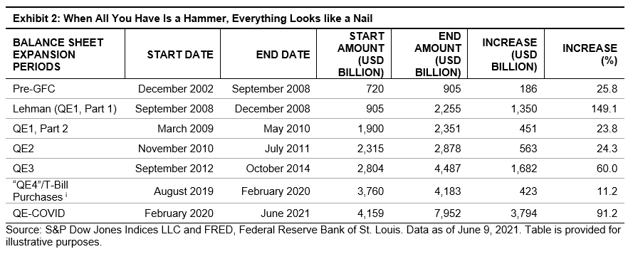
Since the Global Financial Crisis, the U.S. Federal Reserve has actively expanded its balance sheet in an effort to keep markets functioning smoothly and help offset economic downturns. While emergency measures may have been warranted at times, the Fed’s seemingly perpetual support (see Exhibits 1 and 2) has been controversial in many quarters.

The Fed’s go-to counter argument has been that inflation remained well under control, and, in fact, for many years was below their 2% target. While there may be some dislocations in capital allocation, in general, keeping interest rates low makes credit more accessible to individuals and businesses and the lack of inflation limits harm, making easy money policies a net positive.

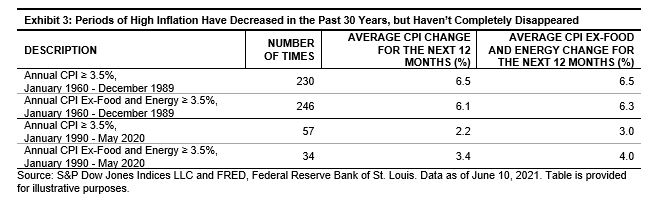
However, the most recent data showed a dramatic uptick in inflation, with a year-over-year Consumer Price Index (CPI) increase of 4.2% in April 2021 and 5.0% in May 2021—the highest reading since 2008. Even excluding the more volatile food and energy sectors, inflation over the previous year was 3.8% in May 2021, the highest since 1992. As previous periods of high inflation have tended to persist in the ensuing months as Exhibit 3 shows, the whispers that the Fed should begin rolling back their market interventions have become louder of late.ⁱⁱ

The high numbers from the past few releases were often dismissed as a “base effects” anomaly in the data. Since April 2020’s price level was artificially low due to the global shutdown at the beginning of the COVID-19 pandemic, it was merely a statistical artifact that calculating year-over-year inflation from that starting point would be so high.

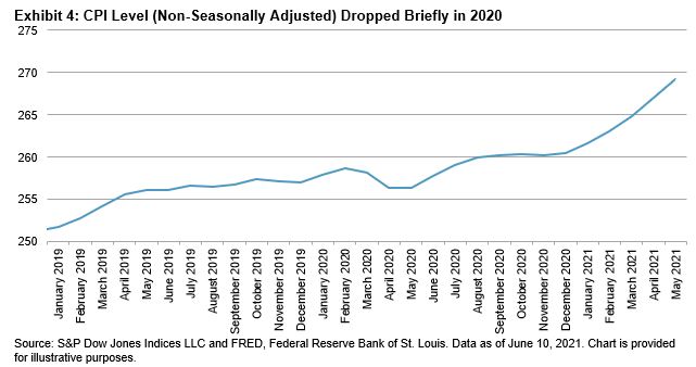
While this is technically accurate, it overlooks the month-over-month (seasonally adjusted) changes. In the past three releases, the month-over-month changes have been 0.6%, 0.8%, and 0.6%. Excluding food and energy, prices have increased 0.3%, 0.9%, and 0.7%. In other words, if the inflation target remains at 2% per year, the Fed has basically used up its annual inflation “budget” within the past three months alone. Unlike the year-over-year series, the changes over the past three months can’t be ignored as coming from an artificially low starting point.

It remains to be seen whether an alternate explanation of “transitory” will hold and the inflation of the past few months is only due to the reopening of the economy and pent-up demand. The Fed’s USD 7 trillion buying binge may yet finally overcome the disinflationary pressures of technological development, demographic changes, and globalization over the past 30 years.

i The Fed vehemently insists this was not actually quantitative easing. The purchase of short-term Treasuries every month was to offset technical dysfunctions in lending markets and not a change in monetary policy. Nonetheless, the “expand the balance sheet” solution hammer applied.

ii The Fed’s 2% target applies to a different measure of inflation, known as the Personal Consumption Expenditure (PCE). The Fed looks at headline PCE inflation over the long-term but tends to focus on core inflation (excluding food and energy) in the short-term. However, in recent years the Fed has talked up the “trimmed mean PCE inflation rate”, which excludes large movements (both positive and negative). The methodological differences between CPI and PCE do not significantly affect the macro issues presented in this post.

In part 1 of this two-part blog series, we discussed the characteristics of the S&P GSCI Dynamic Roll and the two main concerns this index attempts to alleviate, which are negative roll yield and volatility in commodities futures. Diving a bit deeper, we explore the recent performance of a diversified hypothetical portfolio when the S&P GSCI Dynamic Roll is added. Typical allocations to commodities beta range from 2%-20%. After years of commodity underperformance, most market participants’ commodities allocations are no longer at the higher end of the range, despite positive supply/demand catalysts for many individual commodities and the inflation hedging potential of commodities. The May 2021 U.S. CPI reading was +5.0%, a further surprise to the upside after a higher-than-expected 4.2% in April. Exhibit 1 shows how adding a 5% allocation of the S&P GSCI Dynamic Roll provided the same risk-adjusted performance over time but with added inflation protection.

Historically, drawdowns have tended to be less severe for the S&P GSCI Dynamic Roll when compared with the broad commodity S&P GSCI. Exhibit 2 shows the performance of the S&P GSCI Dynamic Roll during the recent market corrections—the initial COVID-19 lockdown in 2020, the 2014 oil price collapse, and during the Global Financial Crisis. During last year’s pandemic lockdown-induced sell off, the headline S&P GSCI fell by more than 50%, while the S&P GSCI Dynamic Roll had a drawdown of 37%, in line with the drop in the S&P 500^®. By not always holding exposure in the most active near-dated futures contracts, the downside performance is buffered because exposure is further out the futures curve in less volatile contracts and contracts that do not reflect spot supply and demand dynamics. The S&P GSCI Dynamic Roll weathered the storm better than other broad commodity market exposures.

For more information on this increasingly popular index strategy, visit our website to learn more. For a more detailed look at the S&P GSCI Dynamic Roll, be sure to read part 1 of this two-part series or check out the S&P GSCI Dynamic Roll Methodology.

U.S. equity markets seemed to undergo a fundamental change of direction in September of last year. Exhibit 1 illustrates the shift; our growth indices, which had outperformed value handily through the end of August, have lagged ever since. The spreads between growth and value are even greater when we compute them using our Pure Growth and Pure Value indices.

Do the strength and longevity of the value rally suggest that it must be near its peak?

To answer directly—we don’t know. Whether value continues to outperform growth or suffers a reversal is a function of numerous exogenous variables, prominently including the course of inflation, the level of interest rates, and the prospects for growth as the economy recovers from last year’s shutdowns. History does, however, let us make two observations about the nature of past value rallies.

First, as Exhibit 2 illustrates, some historical value rallies have lasted far longer than nine months. Since 1995, there have been six cycles when value outperformed growth. The shortest lasted only six months (between February and August 2009). On the opposite side of the ledger, value outperformed for more than four years between 2003 and 2007. So the nine-month duration of the current rally is meaningless in itself.

Second, when value has outperformed historically, its outperformance has accrued smoothly. Exhibit 3 illustrates this for the 2003-2007 value rally, although similar graphs could be (and have been…) drawn for the other periods of value dominance. It’s conceptually possible that, although value outperformed for more than four years, most of the outperformance occurred in the early months, with only a small dollop for latecomers. It turns out that this was not the case; early investors did not reap a disproportionate share of value’s gains.

We don’t know for how much longer value will outperform growth. We don’t know what the ultimate margin of outperformance will be. But the current nine-month cycle is not remarkably long by historical standards, and if it keeps going, history gives us reason to believe that outperformance in the next period can be as good as it was initially.

Launched just over 10 years ago, the S&P GSCI Dynamic Roll was the first dynamically rolling commodity futures index to be offered by a major index provider. What does it mean to dynamically roll? Exhibit 1 describes the process in detail. Employing a flexible monthly futures contract rolling strategy, the S&P GSCI Dynamic Roll is designed to alleviate the negative impact of rolling into contango, to benefit from backwardation, and potentially to lessen volatility while offering investors liquid, broad-based commodity exposure. Contango and volatility are the most cited reasons why market participants tend to steer away from commodities, despite the potential inflation protection and diversification benefits of including commodities in a diversified portfolio. The S&P GSCI Dynamic Roll may help to mitigate these concerns.

Roll yield or carry can add or detract from commodity returns. Any commodity investment product that uses commodity futures as the underlying instrument must continually reinvest, or roll, from expiring nearer-dated contracts into longer-dated contracts to maintain uninterrupted exposure to the respective commodity. If the futures curve is upward sloping (in contango), the roll yield will be negative. If the futures curve is downward sloping (in backwardation), the roll yield will be positive. When the futures curve is in contango holding a position further along the futures curve at a point where the curve is less steep, the negative carry is reduced each time the position is rolled, as opposed to staying in the most near-dated contracts with the steepest contango structure. Exhibit 2 illustrates the steep contango we witnessed in the crude oil market at the start of the pandemic lockdowns in 2020. The S&P GSCI Dynamic Roll was further out on the curve (yellow) than a typical near-dated exposure (navy), where the contango was steepest, thereby reducing the impact of the negative roll yield. In contrast, in March 2021, the crude oil market was in backwardation, and it was advantageous for investors to hold positions at the front of the futures curve.

With many of the 24 commodity constituents of the S&P GSCI in backwardation in 2021, a positive catalyst in the form of a positive roll yield is one of the current reasons to look at commodity exposure. After years of negative roll yields, investors are being rewarded for holding commodity exposure. The S&P GSCI Dynamic Roll is designed to benefit from backwardation by holding positions at the front of the futures curve.

With the contango situation explained, we’ll move on to the volatility in commodities. As we’ve discussed in several prior blogs,¹ commodities are typically the most volatile asset class, leading some risk-averse market participants to stay away. The S&P GSCI Dynamic Roll is designed to be able to hold positions further down the futures curve, limiting exposure to more volatile, near-dated or spot prices. Exhibit 3 illustrates the historical performance of the S&P GSCI Dynamic Roll versus the headline S&P GSCI and other popular alternative commodity beta indices.

Looking for a broad-based, long-only commodity benchmark this year? The S&P GSCI Dynamic Roll may be a better, less-volatile way to gain commodity exposure in 2021. Check out our new Commodities theme page for more information on our indices and timely research to deepen your knowledge of commodities.

¹ https://www.indexologyblog.com/category/commodities/#categories

The Chinese financial market has continued to evolve and mature over the past decade. More and more domestic Chinese investors are starting to take note of investment opportunities from global markets. What are the potential benefits of allocating globally for Chinese investors? In this blog, we will use the CSI 300 Index as a proxy for the China A-shares equity market and the S&P 500^® as a proxy for the U.S. equity market to illustrate that investing globally may provide diversification benefits and could improve risk-adjusted return.

Diversification

As long as two assets are not perfectly correlated, combining them may reduce a portfolio’s overall standard deviation, a common measure of risk.

Despite rising in recent years, the historical correlation of returns between China A-shares and U.S. equity markets has generally been below 0.5 (see Exhibit 1). The low correlation suggests a potential reduction in portfolio volatility when adding U.S. equities to a portfolio of only China A-shares.

Risk-Adjusted Return

On a rolling 10-year basis from Dec. 31, 1994, to March 31, 2021, the U.S. market had a higher risk-adjusted return than the China A-shares market during most periods.

This is driven primarily by different volatility levels observed in the two markets. The China A-shares market was significantly more volatile than the U.S. market, despite a meaningful downward trend in volatility over the past five years.

Looking at absolute return, the U.S. and A-shares markets showed distinct cycles. The average rolling 10-year return for China A-shares was 8.42%, versus 6.98% for U.S. equities.

BLENDING THE CSI 300 INDEX AND S&P 500

Exhibits 3a and 3b show the historical risk/return profiles of hypothetical blended indices created from combinations of the CSI 300 Index and S&P 500 ranging in 10%-20% increments, assuming a monthly fixed-weight rebalance. In the past 3, 5, and 10 years, a hypothetical blended index with weighting to the S&P 500 not only reduced the blended index’s standard deviation but also increased the annualized compounded performance.

Between 2005 and 2020, increasing weights to the S&P 500 improved risk-adjusted returns for the blended index; the reduction in standard deviation more than offset the impact of lower performance. The in-sample optimal allocation of 77% U.S. and 23% China A-shares in the blended index generated a risk-adjusted return of 0.75, higher than both the standalone S&P 500 (0.67) and CSI 300 Index (0.47).

CONCLUSION

Historically, Chinese investors’ allocation to global equities, including U.S. equities, has been low. By underallocating to U.S. equities, Chinese investors have less diversification. Increasing exposure to the U.S. equity market may result in improved risk-adjusted return for Chinese investors. For more details, please refer to Why the S&P 500 Matters to China.