Indexology^® Blog

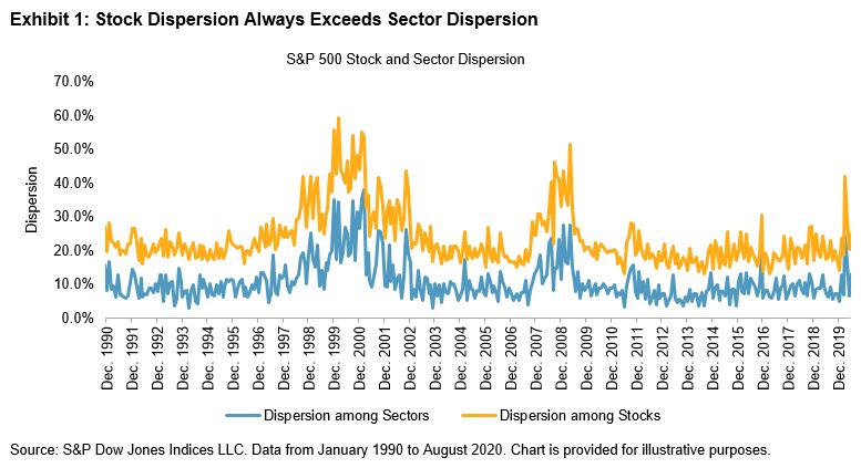
The S&P 600^TM has outperformed the Russell 2000 since its launch in 1994. From Dec. 31, 1994, to Aug. 30, 2020, the S&P SmallCap 600 had an annualized return of 11.77% (with an annualized volatility of 18.96%) versus the Russell 2000’s annualized return of 10.49% (with an annualized volatility of 19.70%).

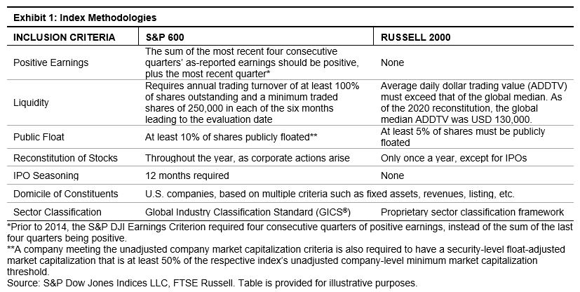
The historical performance divergence is due to differences in index construction, as shown in Exhibit 1. Notably, the inclusion criteria of positive earnings, liquidity, and public float result in the constituents of the S&P SmallCap 600¹ being more profitable, more liquid, and more investable than those of the Russell 2000. In this blog, we explore the validity of profitability, liquidity, and investability screening in index construction.

To attest the overall impacts of profitability, liquidity, and investability, we compare the returns of two hypothetical portfolios constructed by dividing the Russell 2000 (R2000)² universe:

Group 1: Consists of securities that satisfy criteria of profitability, liquidity, and investability as defined for the S&P SmallCap 600.

Group 2: Consists of securities that are not included in Group 1.

For each group, we form equal-weighted and cap-weighted portfolios. Similarly, we also weight the universe equally and by market cap. To show the robustness of our findings, we present the results of the equal-weighted and cap-weighted portfolios. The portfolios are rebalanced monthly.

Equal-Weight Results

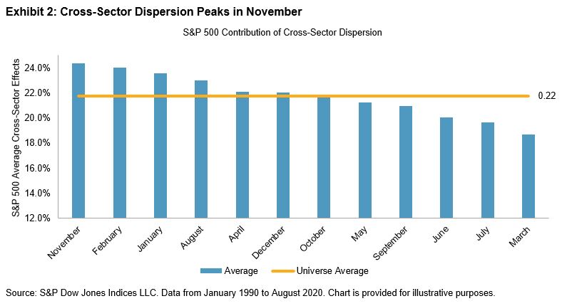
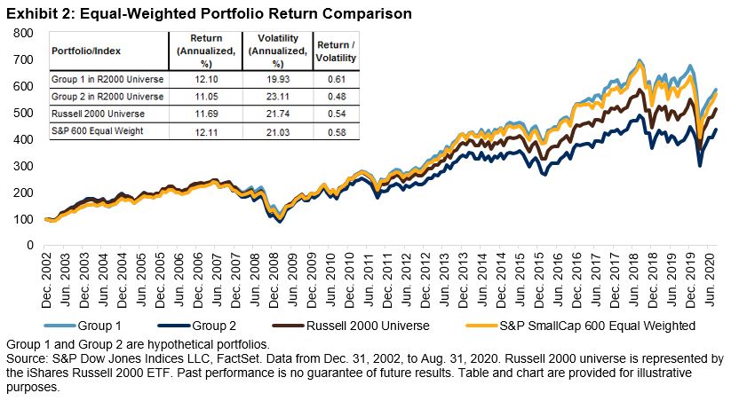
During the period studied, about 700 companies in the Russell 2000 universe would have been in Group 1 and about 1,300 companies in Group 2. Exhibit 2 shows that Group 1 outperformed both Group 2 and the Russell 2000 universe in terms of total return and risk-adjusted return. Such findings indicate that more profitable, liquid, and investable companies tend to outperform their peers in the Russell 2000 universe.

Another important finding is that S&P SmallCap 600 Equal Weighted Index had similar returns to Group1 and naturally outperformed the equal-weighted Russell 2000 universe. The S&P SmallCap 600 Equal Weighted Index achieved its outperformance by using the inclusion criteria of profitability, liquidity, and investability and using only 600 stocks versus 2,000 stocks in the Russell 2000.

Cap-Weighted Results

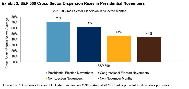
Exhibit 3 shows that the cap-weighted portfolio of profitable, liquid, and investable small-cap securities outperformed the portfolio of other members in the Russell 2000 universe and the underlying Russell 2000 benchmark. Once again, the S&P SmallCap 600 had practically the same returns as Group 1 in the Russell 2000 universe and outperformed the Russell 2000.

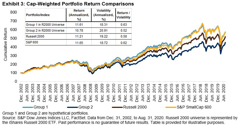
All else equal, the outperformance in the small-cap space came from companies that are profitable, liquid, and investable (Group 1), as captured by the S&P SmallCap 600. Composed of a fraction of stocks in the small-cap universe, the S&P SmallCap 600 could be easier to implement. In sum, the S&P SmallCap 600 is the model benchmark in the small-cap space.

¹ For more detailed index methodology information, please refer to Brzenk, P., W. Hao, and A. Soe. “A Tale of Two Small-Cap Benchmarks: 10 Years Later.” S&P Dow Jones Indices. 2019.

² We use the holdings of iShares Russell 2000 ETF (ticker: IWM) as a proxy for the Russell 2000 universe. Our testing period ran from December 2002 to December 2018 due to the quality of IWM holding data improving after December 2002.

How can the relationship between sectors and factors help investors identify market regime changes and inform allocations? S&P DJI’s Anu Ganti and Hamish Preston take a closer look at market trends through the lens of S&P Composite 1500^® data.

Learn more: https://www.spglobal.com/spdji/en/research/article/the-sp-composite-1500-an-efficient-measure-of-the-us-equity-market/

The current low interest rate environment is forcing many investors to reassess their risk tolerances. Typically, fixed income investors have three main options when trying to “reach” for yield: 1. Move down in credit quality (i.e., take on more credit risk); 2. Increase duration (i.e., take on more interest rate risk); or 3. Move to alternative assets (i.e., those that can potentially incur other illiquidity and lockup provisions). Of course, all of these options pose the same question: Is the incremental yield worth the additional risk?

Staying within the U.S. fixed income asset class, Exhibit 1 shows the broad credit characteristics most investors are currently facing. As expected, a move from BBB investment-grade corporate bonds to BB “junk” bonds produces a 174 bps pick up in yield; however, investors must be willing to tolerate a significant deterioration in credit quality, as well as an exponential increase in default risk. Interestingly, the S&P National AMT-Free Municipal Bond Index has a taxable equivalent yield (TEY) that is 17 bps higher than the yield-to-worst of the S&P U.S. Investment Grade Corporate Bond A Index, offers higher credit quality (AA- versus A), and has a historical default probability of nearly 0%.

For investors uncomfortable with taking on additional credit risk or interest rate risk, a laddered approach presents an alternative. Bond laddering is a mechanism widely used by the investment community to mitigate the potential risks related to buying individual bonds. A ladder helps smooth out the effect of fluctuations in interest rates because there are bonds maturing every year based on the number of rungs in the ladder. When a bond matures, an investor could reinvest that principal in a new longer-term bond at the end of a ladder. Investors may then benefit from a new, higher interest rate, while maintaining the length of the ladder. As shown in Exhibit 2, instead of buying one bond with a six-year maturity, investors can allocate to six different bonds, whereby each bond matures at a different year throughout the six-year horizon.

Investors determine how many rungs their municipal bond ladder should have based on their time horizon. If the goal is to keep the bond ladder in place over time, then as the earliest bond matures, the ladder strategy replaces it with a bond of equal principal at the longer end of the maturity ladder (see Exhibit 3).

The strategy illustrated in Exhibits 2 and 3 allows for construction of a diversified portfolio of bonds from different issuers at each rung of the ladder. Taking this concept a step further, investors have the option of using ETFs that have been specifically designed to incorporate this same structure.

S&P Dow Jones Indices produces a series of indices that seek to track the municipal bond market: the S&P AMT-Free Municipal Series Indices (see Exhibit 4). These indices were designed to reflect the characteristics of a diversified group of bonds that are all high quality, fixed rate, non-callable, and tax exempt. Additionally, each index in the series is composed exclusively of municipal bonds that mature in the stated year, allowing for targeted return of principal and potential reinvestment.

As shown, bond ladders offer a simplified approach when navigating uncertain interest rate environments, while also providing relatively predictable levels of income. For more details and examples of how implementing a laddering strategy using indices can offer additional benefits, please be sure to read the recently updated education piece: Bond Laddering with the S&P AMT-Free Municipal Series Indices.

Markets expect elevated volatility surrounding the U.S. Presidential election, now just six weeks away. The VIX futures curve currently peaks in November, but as long ago as April a close observer could detect expectations of electoral volatility. Increased volatility may create an unusual opportunity for sector allocators.

To understand why, we need to remember that volatility is directly connected to dispersion, which measures the spread among the returns of an index’s components. When volatility goes up, dispersion tends to rise as well, as the gap between winners and losers widens; we saw a spectacular example of this in the first quarter of 2020. The greater the spread, the greater the opportunity to add (or subtract) value.

Dispersion can be measured at various levels of granularity—for example among stocks or sectors in the S&P 500^®, as illustrated in Exhibit 1. Obviously, the spread among the returns of 500 stocks will be greater than the spread among the returns of 11 sectors. (The larger spread is partially offset by the superior capacity of sector-based funds.)

The total dispersion of the S&P 500 (at the stock level) can be decomposed into the average dispersion within each sector and the dispersion across sectors. The nature of the relationship will be familiar to anyone who remembers high school geometry: the square of total dispersion is approximately equal to the sum of the squares of within-sector and cross-sector dispersion.

Over time, cross-sector dispersion has accounted for approximately 22% of the market’s total dispersion. But the overall average masks substantial calendar variation. As Exhibit 2 shows, the importance of sector dispersion peaks in November and is relatively low in March.

And as it turns out, some Novembers are more significant than others. Specifically, in 71% of the Novembers when U.S. Presidential elections took place, the importance of cross-sector dispersion in the S&P 500 was greater than average, as shown in Exhibit 3. In off-year elections (with only Congressional and Senate seats at stake, but not the White House), sectoral importance also rises, although not to the level of Novembers with a Presidential contest.

Dispersion, it’s important to remember, is a double-edged sword. Higher dispersion raises the stakes for active managers, in both directions: if dispersion is high, correct stock or sector picks will pay off more, and incorrect picks will underperform by more. History tells us that the contribution of sectors to total dispersion is likely to rise in the next six weeks, which means that the importance of skillful sector picks will increase. For investors with a genuine ability to rotate across sectors tactically, November could be a month of unusual opportunity.

Many market participants invest in small-cap equities seeking high-growth potential and portfolio diversification. In this blog, we will examine how growth factors performed in Australian small-cap equities by measuring the hypothetical top-quintile portfolio returns for three growth factors with long- and short-lookback periods, including 12- and 6-month price momentum, 3- and 1-year earnings growth, and 3- and 1-year sales growth based on the S&P/ASX Small Ordinaries index universe.¹

For the period from April 20, 2001, to June 30, 2020, the 12- and 6-month price momentum were the best-performing factors, with 8.83% and 7.29% annualized excess returns, respectively, compared with the S&P/ASX Small Ordinaries (see Exhibit 1). The 3- and 1-year earnings growth factors had relatively modest annualized excess returns of 2.10% and 2.90%, respectively, with a tracking error of nearly 7%, which was the lowest among the other growth factors studied. The 3- and 1-year sales growth factors recorded the smallest annualized excess returns at 1.29% and 0.09%, respectively, compared with the S&P/ASX Small Ordinaries. The earnings growth factor had a beta close to 1, whereas sales growth and momentum had higher betas at 1.2 relative to the S&P/ASX Small Ordinaries.

For the price momentum and sales growth factors, the portfolios with longer lookback periods (12-month price momentum and 3-year sales growth) had higher risk-adjusted returns and information ratios than those of the portfolios with shorter lookback periods (6-month price momentum and 1-year sales growth), though the earnings growth portfolios did not follow the same pattern. Overall, the portfolios with longer lookback periods witnessed lower portfolio turnover. The 3-year earnings growth, 3-year sales growth, and 12-month momentum portfolios recorded one-way annualized portfolio turnovers of 91.8%, 79.7%, and 120.3%, whereas the 1-year earnings growth, 1-year sales growth, and 6-month momentum portfolios had much higher turnover rates of 120.2%, 111.5%, and 158.2%, respectively. Considering the excess returns and replication cost of the portfolios, constructing growth portfolios with longer lookback periods tended to deliver higher returns historically.

Over the period studied, we noticed the outperformance of various growth factors was not consistent across different periods of time (see Exhibit 2). Though momentum was the best-performing factor across the observed horizon, it tended to underperform the S&P/ASX Small Ordinaries and other growth factor portfolios when market regimes transitioned from a bear or time-correction phase to a bull phase. This trend was visible in 2004 (following the war in Iraq), in 2009 after the Global Financial Crisis (GFC), and in 2016 and 2018.

On the other hand, sales growth portfolios did not deliver pronounced excess returns over the entire period, but they tended to perform better during bull markets, which were seen during the pre-GFC period (2006-2007), post-GFC period (2009), and between 2016 and 2019. The sales growth portfolios also had the highest portfolio betas, which accentuated their outperformance during the stock market bull runs.

The earnings growth portfolios had a higher tendency to better perform during market distress, especially in the 3-year earnings portfolio. During the European sovereign debt crisis from 2011-2013, the 3-year earnings growth portfolio delivered pronounced excess returns, and in the recent pandemic crisis (the first half of 2020), both the earnings growth portfolios outperformed the S&P/ASX Small Ordinaries. During volatile periods, market participants may look for safer investments by tilting their portfolios toward profitable companies with robust earnings growth.

From these observations, we conclude that the three growth factor portfolios of price momentum, earnings growth, and sales growth clearly delivered risk premia over the long term in Australian small-cap equities, with the most pronounced excess returns from the price momentum factors, though these growth factors played out differently across changing market regimes over the period studied. We also noted that growth factors with shorter lookback periods did not necessarily deliver better absolute and risk-adjusted returns compared with their respective portfolios with longer lookback periods, but they recorded higher portfolio turnover, hence higher replication costs. This implies that growth factors with longer lookback periods may be more effective for constructing growth factor portfolios in Australian small-cap equities.

¹   Z-scores for each of the growth factors are computed for all constituents in the S&P/ASX Small Ordinaries. Companies ranked in the top quintile by their factor z-scores form the respective growth portfolios, which rebalance semiannually on every third Friday of April and October. All portfolios are weighted by their float-adjusted market caps that are tilted by factor z-scores, with individual constituent weights capped at 10%. As earnings and sales growth cannot be evaluated for companies with negative values in the base year, they are ineligible to be part of the earnings and sales growth portfolios.