Indexology^® Blog

In my last blog, we discussed the performance characteristics of the S&P/ASX BuyWrite Index. We will now focus on the income-generating feature of this index.

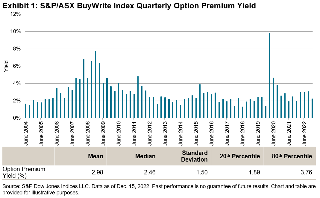
As a reminder, a covered call strategy involves selling a call option against an asset that is already owned by the option writer. A systematic long-term covered call strategy generates a steady income stream through the accumulation of option premiums. The S&P/ASX BuyWrite Index employs such a strategy by selling quarterly at-the-money calls against a long position in the underlying S&P/ASX 200. Since its launch in 2004, the index has achieved an average quarterly option premium yield of 2.98%, with yields peaking during the bear markets of the Great Financial Crisis of 2008 and March 2020 (see Exhibit 1).

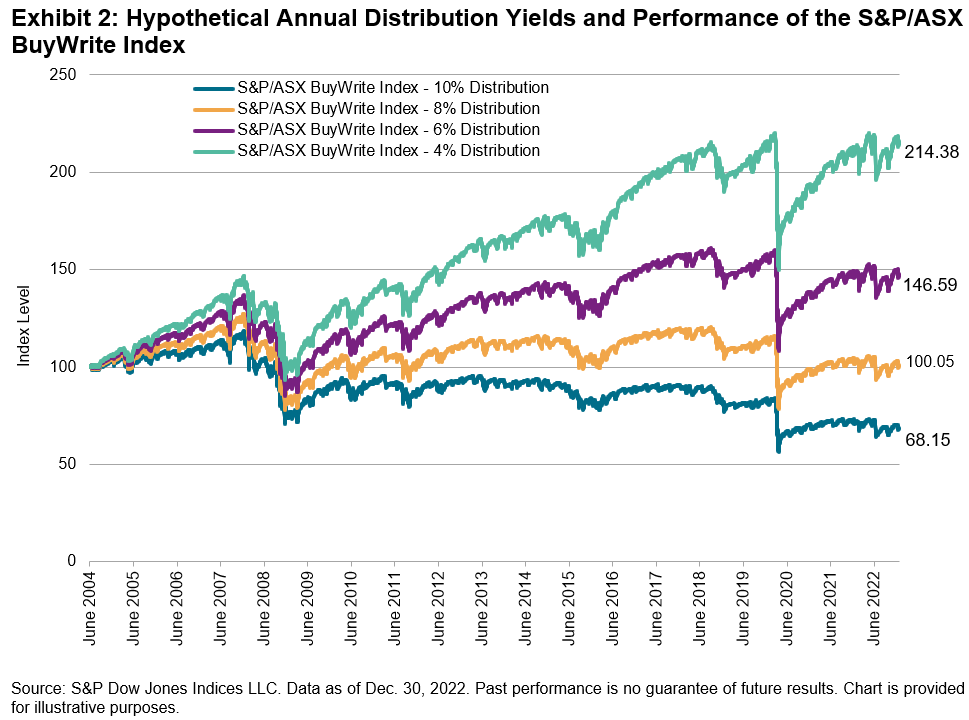
The premiums and dividends generated by the S&P/ASX BuyWrite Index are reinvested into the long equity position—the underlying S&P/ASX 200. In a hypothetical scenario in which the premiums and dividends are distributed instead of reinvested, the index would have been able to achieve an annual distribution yield of 8% across its 18-year history without losing its initial principal value (see Exhibit 2). This represents a potentially valuable source of income.

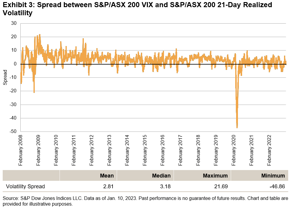
Theoretically, the income-generating feature of this type of strategy is associated with the spread between implied and realized volatility. Implied volatility can be defined as the market’s prediction of an asset’s future volatility, while realized volatility represents the volatility that actually occurred. The S&P/ASX BuyWrite Index is able to capture the risk premium that arises from the discrepancies between these two measures of volatility. In general, a covered call strategy pays off when the implied volatility of the index—as measured here by the S&P/ASX 200 VIX—is greater than its realized volatility. On average, this has been the case since 2008 (see Exhibit 3). Since implied volatility is one of the key factors in option pricing, a lower realized volatility allows option sellers to capture higher option prices—premiums—than the realized market conditions would have merited—this phenomenon is known as the volatility risk premium.

In the first seven weeks of 2023, U.S. equities regained a third of the ground lost in 2022 (down 18.1% in 2022 and up 6.5% YTD through February 17, 2023). Exhibit 1 shows that since its last rebalance, the S&P 500^® Low Volatility Index, which seeks to mute the gyrations of the market in both directions, underperformed the market by 1.3%.

Exhibit 2 shows that volatility has remained meaningfully flat since November 2022, with a 2% increase at the high end for Communication Services, Materials and Real Estate. Consumer Discretionary and Energy hold their places as the most volatile sectors of the S&P 500.

Despite the relative calm in the risk landscape, Low Volatility’s latest rebalance, effective after the market close on Feb. 17, 2023, brought some significant changes.

Real Estate has never quite regained its pre-COVID presence, but as Exhibit 3 shows, this rebalance reduced Low Volatility’s allocation to the sector to 1%. Utilities also pared back its weight by 3%. The slack went mainly to Health Care and Financials, which added 5% and 2%, respectively. Given the minimal changes in volatility at the sector level, the shifts in sector allocations for the low volatility index indicate there might be more going on idiosyncratically within the sectors.

Disruptions to global supply chains have put the global shipping market in the spotlight, highlighting its contribution to international trade and its significance as an important link in the chain of the world economy. One of its sectors is the dry bulk market that involves the transportation of commodities such as iron ore, grains, coal (coking and thermal), bauxite and alumina, and fertilizers. In 2021, dry bulk vessels carried more than 45% of the world’s seaborne trade.

Determinants of Freight Rates

Freight rates are driven by the balance between demand for seaborne trade and the supply of shipping services. The former correlates with world GDP cycles and is affected by prevailing conditions in the related commodity trades. Commodity markets affect the demand for shipping in both the short and long-term. Short-term fluctuations in shipping markets may be caused by the seasonality of some trades (e.g., in agricultural commodities) while long-term fluctuations are due to changes in the economies of the countries that import and export the corresponding commodities. Demand is also affected by the distance over which commodities are transported, known as the “average haul”.¹ Finally, one must also consider random demand shocks caused by, among others, geopolitical events such as the recent conflict in Ukraine.

In contrast to demand, supply depends on the size of the global fleet, utilization rates, and—as witnessed during the COVID-19 pandemic—shocks caused by disruptions to the free movement of people and vessels. Shipping supply increases as new ships are delivered and decreases through the demolition of existing ones. Delivery of a newbuilding order requires a time-to-build and depends on prevailing market conditions as well as capacity in the shipbuilding industry. Equally, supply may be affected by changes in regulations. For instance, new environmental regulations that will come into force in 2024 require a part of the CO₂ emissions from ships to be priced into the cost of freight. As emissions depend on the amount of fuel consumed, which in turn depends on the sailing speed, one way of reducing emissions is via slow steaming which will reduce the supply of ships.

Freight Rates and Commodity Prices

Commodity exposure to freight rates varies by vessel type and trade route but represents a noticeable percentage of the final value of a commodity. For example, freight accounts for up to 20% of the overall cost of iron ore that is exported from Brazil to China. To illustrate further, a recent study by the United Nations Conference on Trade and Development (UNCTAD) has shown that higher dry bulk freight rates, combined with higher grain prices, can contribute to a 1.2% increase in consumer food prices with price increases noticeably higher in middle-income economies whose food imports depend more on dry-bulk shipping.²

Closing thoughts

Shipping provides the most efficient way of transporting bulk commodities over long distances and is thus a very important link in the chain of the World economy. The recent introduction of the S&P GSCI Freight Indices has made these markets accessible with unique risk-return characteristics and low correlation to other financial assets and commodities.

¹ Average haul is the typical distance over which commodities are transported by sea and is measured in tonne-miles, defined as the product of the quantity of shipped cargo times the transportation distance.

² UNCTAD 2022 Review of Maritime Transport, p. xxii. Available on: https://unctad.org/system/files/official-document/rmt2022_en.pdf

With more than $7 trillion tracking the S&P 500 alone, we estimate that index funds now encompass between a quarter and a third of the capitalization of the U.S. equity market. This extraordinary growth must surely rank as one of the most important developments in contemporary financial history.

When will it end? For at least the last five years, critics of indexing have argued that the growth of passive management is a “bubble” and, like all investment bubbles, destined to end with weeping and gnashing of teeth. We saw the Information Technology sector peak in 2000, and Financials in 2007. Might we now be approaching what some analysts characterize as “peak passive?”

What index funds today and technology stocks in the late 1990s have in common is that both have attracted large inflows. But that is where the similarity stops. The technology bubble was driven by active decisions, as investors allocated more and more weight to one segment of the market. The growth of indexing is driven by investors eschewing active decisions—in other words, by recognizing that most active managers underperform most of the time. As the technology bubble inflated, portfolios became more concentrated; as assets move from active management to index funds, portfolios become more diversified.

Despite these obvious benefits, we concede that indexing’s impact on market efficiency is ambiguous. It’s fair to describe the typical index portfolio as a price taker rather than a contributor to price discovery. This means that the valuation of index constituents is ultimately decided by active managers (and some factor indices) whose trades are motivated by their own research. And indexers do contribute to market efficiency indirectly, by taking assets from the least capable active managers, thus increasing the influence of their more astute competitors.

All this means that the idea of “peak passive,” while computationally unclear, isn’t conceptually wrong. But understanding where the peak might be requires us to distinguish between passive assets under management and passive trading.

Comprehensive cap-weighted index funds trade relatively little in comparison to active managers. Exhibit 1 shows that, on reasonable assumptions, if indexers own a third of the market’s assets, active managers will still do 91% of all trading. Under these assumptions, index AUM share must rise above 83% before active managers’ share of trading drops below 50%. And even at that level, there’s no a priori reason to assume that market efficiency would be impaired. (After all, active research is not unfailingly prescient.)

How will we know, at some future date, that markets are no longer sufficiently efficient? Presumably one of the indicia of market inefficiency would be a sufficiently large number of mispriced stocks, so that the value of successful active management would increase. This is a plausible outcome. But remember: the only source of outperformance for the outperformers is the underperformance of the underperformers. Active investment management remains a zero-sum game.

Even if we do approach peak passive, therefore, the active manager’s life will be no easier, and the benefits of indexing will be no less.

Why did indexing take root and how has it grown so far so fast? S&P DJI’s Craig Lazzara and Anu Ganti take a closer look at why indexing works, the size of the passive market today, and the historical savings linked to indexing.