Get Indexology® Blog updates via email.

In This List

The bad kind of volatility?

What About the Debt of PEMEX?

Will Housing Be Dealt Another Bad Hand?

Big Picture: Bonds Have Held Up Well

Commodities Post 4th Biggest 2-Day Gain Since 1970

The bad kind of volatility?

Contributor Image
Tim Edwards

Managing Director, Index Investment Strategy

S&P Dow Jones Indices

Markets across the globe were rocked by volatility from sources new and old last month.

The old was a play-by-play repeat of the “taper tantrum” as capital fled from emerging markets in anticipation of a September date for the first rise in U.S. rates since 2006.

The new was triggered by evidence that the rollercoaster performance of equity markets in China (previously judged to be the result of high-octane day-traders learning the pain of a margin call) was also the first sign of a stall in the world’s economic growth engine.

August was a month of records – the VIX® recorded its biggest ever monthly gain, the average correlation between European equities rose to their highest ever.

VIX & 350 C

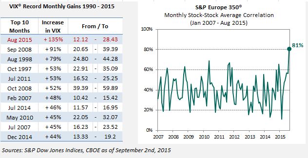
Why such high correlations in Europe, and such dramatic gains in VIX?  The answer is twofold.

  1. August is typically a quiet month. When something “happens”, it tends to dominate.  The only other major market to record a monthly stock-to-stock correlation in the 80’s was the U.S. S&P 500 during August 2011 (at that time, the failure to agree the budget threatened a technical default on U.S. Treasuries).
  1. There still remains very little dispersion. The world’s equity markets have been feeding on vast amounts of global, fiscal stimulus.  Our limited historical data suggests that such environments result in very little distinction between the performances of different stocks.  When every stock follows the same story, dispersion falls.  The impact of this is there is less diversification in stock indices; their correlations rise and index volatility rises with it.

This makes for a fragile environment.  As we saw in the “Flash Crash” of 2010, when correlations are high and dispersion is low, even a small and otherwise minor market disruption can have catastrophic consequences. This is the “bad” kind of market volatility, with few stocks providing refuge and little benefit to diversification. Be careful out there…

The posts on this blog are opinions, not advice. Please read our Disclaimers.

What About the Debt of PEMEX?

Contributor Image
Jaime Merino

Former Director, Asset Owners Channel

S&P Dow Jones Indices

Since 1938, the state has been doing all the work. PEMEX was the only company managing the exploration, exploitation, and commercialization of oil but with the energy reform, things will change. PEMEX is the biggest company in Mexico, with sales over USD 123 billion and total assets over USD 156 billion as of 2013. Mexico recently opened the market for more participants through the tenders that started with “Ronda Uno” (Round One) in July 2015. In this first phase, only two blocks out of 14 were awarded, which was not what the Ministry of Energy was expecting (between 30%-50%). The next phase of Ronda Uno will be on Sept. 30, 2015, with five different contracts to be awarded in nine different blocks for drilling.

The global economy, especially China, has not helped with this. Year-over-year, Mexican crude fell 63.05%, from USD 91.22 to USD 33.71 (as of Aug. 24, 2015). Exhibit 1 shows the price of Mexican crude over the past five years.

Capture

But, What About the Debt of PEMEX?

Nowadays, PEMEX issues debt in pesos, dollars, and euros. By the end of 2013, the debt in U.S. dollars represented 79% of the company’s total debt. Focusing on the local debt and using local information, we created four indices classified by: fixed-rate debt, inflation-linked debt, floating-rate debt, and a separate index comprising the other three. For the inflation-linked index, the cumulative returns were -2.50% YTD, and -1.04% for the one-year period. During the same time period, the fixed-rate debt returned only 1.52% YTD and 2.05% year-over-year, as shown in Exhibits 2 and 3.

Capture

Capture

The total local debt was distributed into 14 issues (not including the PEMEX 09U series or ABS), with a total market value of USD 13.25 billion (as of July 31, 2015, using a spot price of MXN 16.1088), where 59% of the total is represented by fixed-rate bonds and 26.74% matures in 2024. Exhibit 4 shows the distribution of the different rates and Exhibit 5 the maturity in billions of U.S. dollars in market value.

Capture

Capture

Finally, if we think about a peer for PEMEX —not from an oil perspective but from the perspective of a quasi-sovereign company in Mexico—the Federal Electrical Commission (CFE) is the first name that comes to mind. With six different types of bonds (excluding ABS) and USD 4.06 billion of market value, PEMEX represents 56% of the S&P/Valmer Quasi-Sovereign Bond Index, while CFE represents 28%. Comparing the fixed-rate bonds of these two, Exhibit 6 shows how PEMEX has underperformed CFE. Moreover, we can compare them with some of the indices of the S&P/Valmer Indices, and we can see also how PEMEX has underperformed year-to-date and over the one- and three-year periods.

Capture

The posts on this blog are opinions, not advice. Please read our Disclaimers.

Will Housing Be Dealt Another Bad Hand?

Contributor Image
Marya Alsati

Former Product Manager, Commodities, Home Prices, and Real Assets

S&P Dow Jones Indices

On Monday, Aug. 24, 2015, the global stock market tumbled, with the Dow Jones Industrial Average® losing 1,000 points in seconds. We have seen similar turbulence in the equity markets in 1987, 1997, 1998, 2007, and 2008.

We know that the stock market is an important leading indicator, as it reports on the health of companies’ earnings estimates and the health of the global economy. Housing prices can also be considered leading indicators, as a decline in housing prices can be representative of excess supply and inflated prices.

The S&P/Case-Shiller Home Price Indices use the repeat sales methodology, which has the benefit of directly measuring changes in home prices by only including homes that have been sold twice. The indices are calculated monthly, using a three-month moving average. Index levels are published with a two-month lag.

I want to use this post to see if the sharp declines in equity prices (using the S&P 500® ) are reflected in the S&P/Case-Shiller Home Price Indices, and, if so, in what time frame and at what magnitude? The dates evaluated are depicted in Exhibit 1.

Capture

Exhibit 2 charts the levels of the S&P 500 against the levels of the S&P/Case-Shiller U.S. National Home Price Index.

Capture

While the indices moved in the same general direction, one clear difference was that the volatility in the equity market was not reflected in the housing market. The next step was to drill into the returns near the dates of the previous stock market crashes presented in Exhibit 1.

Prior to the stock market crash of 1987, the housing market had been exhibiting modest gains, and it did not turn into negative territory until August 1990, which was a period of recession in the U.S. Between that period and the crash of 1997, out of the 120 monthly return observations, the S&P/Case-Shiller U.S. National Home Price Index only reported 35 declines, and it proceeded to remain positive past the 1997 and 1998 crashes. The index went into negative territory in August 2006 (after a strong upward trend), one year before the August 2007 crash, and it stayed there through the September 2008 crash. It did not turn positive until 2010, and it continued to alternate between months of gains and months of losses until the present. By analyzing this data alone, it appears that the S&P/Case-Shiller Home Price Indices are more sensitive to mass economic crises and recessions than to turbulence in the equity market.

David Blitzer, Managing Director and Chairman of the Index Committee at S&P Dow Jones Indices, summed it up nicely saying, “Stock market correction is unlikely to do much damage to the housing market; a full-blown bear market dropping more than 20% would present some difficulties for housing and for other economic sectors.”

Just as food for thought, Exhibit 3 shows the levels of the S&P 500 and the S&P/Case-Shiller U.S. National Home Price Index against a blended, of the two indices (50% allocation in each index). The blended index enjoyed some benefits from the equity portion, gaining as much as 5.45% in December 1991, but it is less volatile than the equity index as is illustrated.[1]

Capture

[1]   It should be noted that investors cannot invest directly in an index.

The posts on this blog are opinions, not advice. Please read our Disclaimers.

Big Picture: Bonds Have Held Up Well

Contributor Image
Kevin Horan

Former Director, Fixed Income Indices

S&P Dow Jones Indices

August is shaping up to be a negative month for the S&P 500 Bond Index (-0.52% month-to-date and -0.61% YTD), as of Aug. 28, 2015.  Though, for all the drama of this month, attributable to the drop in oil prices (-24% YTD), weakness in the Chinese economy, and a major sell-off in equities, bond returns look relatively stable.  U.S. equities, as measured by the S&P 500, have a total return of -2.07% YTD, (-3.4% price return) as of the same date.

Investors who have been chasing higher yields by moving down in credit will most likely experience a loss this month, as the S&P 500 High Yield Corporate Bond Index has returned -1.26% month-to-date.  The S&P 500 BB High Yield Corporate Bond Index has returned -1.5% month-to-date, while the single B index is down -0.70% month-to-date and the CCC and lower index is down -0.99% month-to-date.  When looking at the year-to-date returns, the riskiest of assets (S&P 500 CCC & Lower High Yield Corporate Bond Index) is still holding up, returning 3.16% after being as high as 4.33% on July 16, 2015.

Higher up the rating scale, the loss has been to a lesser degree.  The S&P 500 Investment Grade Corporate Bond Index has returned -0.46% month-to-date and -0.68% YTD.  The monthly returns by rating bucket are as would be expected, with AAA returning -0.18%, AA -0.26%, A -0.25%, and BBB -0.65% month-to-date.

At the height of this month’s selling, many questions arose about how bonds have performed historically.  Exhibit 1 shows that even in most stressed of times (2008), investment-grade bonds weathered the storm, while high-yield bonds experienced significant losses.  Those losses did not last too long, however, as the lower credits and investment-grade bonds bounced back in performance in December 2008 and did not look back during 2009.

Exhibit 1: Historical Returns
S&P 500 Bond Index and Rating Sub-Indices

The posts on this blog are opinions, not advice. Please read our Disclaimers.

Commodities Post 4th Biggest 2-Day Gain Since 1970

Contributor Image
Jodie Gunzberg

Former Managing Director, Head of U.S. Equities

S&P Dow Jones Indices

As of the close on Aug. 28, 2015, the S&P GSCI Total Return gained 8.98%, the most in 2 days since Jan. 2, 2009.  It was the 4th best gain over 2 consecutive days in the history of the index that has data beginning on Jan. 2, 1970. The bigger 2-day gains are shown in the table below:

Source: S&P Dow Jones Indices LLC. Daily Data from Jan. 2, 1970 - Aug. 28, 2015.
Source: S&P Dow Jones Indices LLC. Daily Data from Jan. 2, 1970 – Aug. 28, 2015.

The high total returns in the world production weighted S&P GSCI were driven by strong oil performance, the biggest component in the index. On Aug. 27, 2015, the S&P GSCI Crude Oil experienced its 8th biggest gain in history, up 10.26%. This was followed by another daily gain of 6.25% to record the 3rd biggest 2-day gain for the S&P GSCI Crude Oil, in its history since Jan. 6, 1987 as shown below:

Source: S&P Dow Jones Indices LLC. Daily Data from Jan. 6, 1987 - Aug. 28, 2015.
Source: S&P Dow Jones Indices LLC. Daily Data from Jan. 6, 1987 – Aug. 28, 2015.

As shown before, rising oil floats all boats, and on Friday 17 of the 24 commodities gained, which is a major improvement from the direction last month when 23/24 commodities recorded negative total returns. However, when looking month-to-date in August, it is not much better with only 3 positive commodities; lead +1.8%, lean hogs +4.2% and gold +3.6%.

Unfortunately for commodities, just because there was a historically large spike, it doesn’t indicate they hit the bottom.

After the 2-day gain of 10.4% on Aug 6, 1990, the S&P GSCI continued to gain 25.7% through Oct. 9, 1990, but lost it all giving up 26.8% by Jan. 18, 1991. It never really picked up again until 1996.

Source: S&P Dow Jones Indices

The two other higher 2-day gains were realized in the 2008-9 time period. The first spike on Jun. 6, 2008 happened before the crash but the second spike happened on the way down. The latter is more interesting to evaluate since the peak only squeezed out an extra 5.3% by July 3, in 2008. However, the 2-day spike ending Jan. 2, 2009, was followed by a decline of 24.2% until the bottom seemed to reached on Feb. 18, 2009.

Source: S&P Dow Jones Indices

While the index rose 85.3% until Apr. 8, 2011, it has now given up 53.8% and has created a new biggest drawdown of 77.5% as of Aug. 26, 2015. It is yet to be seen whether the fall will continue but what is concerning besides the difficult fundamentals is that the volatility is still not historically high. Historically the volatility has spiked, becoming too volatile for investors hence causing them to sell. This has driven  drops in open interest in historical crises that we haven’t seen yet.

Source: S&P Dow Jones Indices. Red line is 90-Day Annualized Rolling Volatility on left axis. Blue line is Index Levels on the right axis.


To hear more expert opinions about commodities, please join us for our 9th annual commodity seminar. 

Source: S&P Dow Jones Indices LLC. Daily Data from Jan. 2, 1970 – Aug. 28, 2015. The launch date of the S&P GSCI was May 1, 1991. All information presented prior to the index launch date is back-tested. Back-tested performance is not actual performance, but is hypothetical. The back-test calculations are based on the same methodology that was in effect when the index was officially launched. Past performance is not a guarantee of future results. Please see the Performance Disclosure at http://www.spindices.com/regulatory-affairs-disclaimers/ for more information regarding the inherent limitations associated with back-tested performance.


The posts on this blog are opinions, not advice. Please read our Disclaimers.