Get Indexology® Blog updates via email.

In This List

For Active Managers, Staying on Top Is Not Enough

What’s inside the S&P China A-Share Factor Indices? The Impact of Style Risk Factors

Performance of Latin American Markets in Q2 2019

Sector Analysis of the S&P MidCap 400®

The Heat Is On for High Yield in July

For Active Managers, Staying on Top Is Not Enough

Contributor Image
Berlinda Liu

Former Director, Multi-Asset Indices

S&P Dow Jones Indices

S&P DJI’s Mid-Year 2019 Persistence Scorecard may offer a hint of encouragement for active fund managers. Performance persistence, measured over the three-year period ending March 2019, rose from prior periods. Among the domestic equity funds that were in the top quartile as of March 2017, 11.36% were able to go on and maintain their top-quartile status in the subsequent two years. This figure is a substantial increase from six months prior (7.09%) or even one year prior (2.33%).

However, further study of these top quartile funds shows that it is not enough for active managers to stay ahead of the game with one’s peers; the challenge of beating the benchmarks has intensified.

Using the same methodology as the S&P Persistence Scorecard, we first identified the domestic equity funds that made top quartile status as of March 2017 according to their annualized returns from the prior three-year period. These are the same top quartile funds that we refer to in this blog. We then compared these funds with the universe of all domestic equity funds and the broad market benchmark, the S&P Composite 1500®.

Our goal was to examine whether the top quartile status of active funds led to future outperformance relative to their peers and to the benchmark.

Only a fraction of these original top quartile funds managed to stay in the same league for the two subsequent consecutive years. However, the final top quartile funds displayed some remarkable characteristics. First, they collectively navigated the seesawing market conditions of the past year better than their peers. As shown in Exhibits 1 and 2, these funds generated approximately three percentage points of extra returns, as measured by the mean and median. On average, their annualized volatility was 0.78 percentage points lower than that of the peer group category. Exhibit 1 also shows that the risk/return profiles of these funds were more homogenous than the peer group category; the standard deviations of return distribution and volatility distribution were smaller in this group of funds.

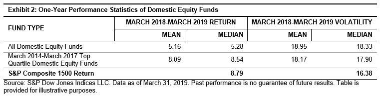
However, the advantage of these top quartile funds disappears once we compare them with the benchmark. The S&P Composite 1500 returned 8.79% with 16.38% volatility during the trailing 12-month period ending March 2019. Compared to the benchmark, the top quartile funds on average returned 70 bps less with 179 bps higher volatility in the same period when compared with the benchmark (see Exhibit 2). In other words, beating the benchmark remained challenging even for managers that ranked high in their peer group category.

For more information on how fund performance persisted, read our latest Persistence Scorecard.

The posts on this blog are opinions, not advice. Please read our Disclaimers.

What’s inside the S&P China A-Share Factor Indices? The Impact of Style Risk Factors

Contributor Image
Liyu Zeng

Director, Global Research & Design

S&P Dow Jones Indices

In our previous blog, our studies indicated that most factor indices in China exhibited distinct return characteristics during up and down markets. To understand the sources that drive differential factor performance, we examined the risk factor exposures and factor impact on the performance of S&P China A-Share Factor Indices[1] based on the Axioma AXCN4-MH China equity factor risk factor model.

As indicated in Exhibit 1, over the period from July 31, 2006, to April 30, 2019, value, small caps, and low volatility were the best-performing risk factors in the China A-Share market. Therefore, exposures to these factors could have a significant impact on portfolio returns.

Different factor indices displayed distinct risk factor exposures (see the Appendix for risk factor definitions). All S&P China-A Share Factor Indices exhibited targeted active factor exposures relative to the eligible universe (see Exhibit 1). Unintended active factor exposures were also observed in various indices. For instance, the S&P China A-Share Short-Term Momentum Index showed strong active exposure to high volatility, expensive valuation, and low dividend yield. The S&P China A-Share Enhanced Value Index had significant active exposure toward large caps, low volatility, and high dividend yield, while the S&P China A-Share Dividend Opportunities Index displayed significant active exposure to cheaper valuation and high profitability. The S&P China A-Share Quality Index exhibited an active tilt toward expensive valuation, high dividend yield, and low beta, while the S&P China A-Share Low Volatility Index had unintended active exposure toward high dividend yield and cheaper valuation.

To understand the main drivers of portfolio performance, we decomposed the active returns of portfolios into different style risk factors, industry factors, and stock-specific risks.

As shown in Exhibit 2, over the same period, most of the underperformance of the S&P China A-Share Short-Term Momentum Index was driven by its exposure to high momentum, high volatility, and expensive valuation. Small caps was the only style factor that had significant positive impact on active returns.

As expected, the value factor was the main driver of the outperformance of the S&P China A-Share Enhanced Value Index. Its unintended exposure to low volatility and high dividend yield also had a positive contribution to its active returns.

The excess returns of the S&P China A-Share Dividend Opportunities Index were mainly driven by its targeted exposure to high dividend yield and associated exposure to cheaper valuation, low volatility, and small caps.

Consistent with the design of the quality index, profitability and low leverage contributed positively to its active returns. However, the unintended exposure to high volatility and expensive valuation generated negative return contribution historically.

Unsurprisingly, low volatility was the main source of the active returns of the S&P China A-Share Low Volatility Index. Its unintended biases to cheaper valuation and small caps had a significant contribution to its outperformance as well.

As we can see from this risk attribution analysis, different factor portfolios had distinct factor exposures, which might drive performance differently. Decomposing the source of active returns can be useful for investors to understand the behavior of factor portfolios in different market environments.

[1]   All portfolio constituents are drawn from the combined universe of the S&P China A BMI Domestic and S&P China A Venture Enterprises Index except for the S&P China A-Share Dividend Opportunities Index. To ensure investability, eligible stocks must have a float-adjusted market capitalization no less than RMB 1 billion and a three-month average daily value traded not below RMB 20 million. The S&P China A-Share Enhanced Value Index, S&P China A-Share Short-Term Momentum Index, and S&P China A-Share Quality Index include the 100 stocks with the highest factor scores, and the stocks are weighted by their score-tilted market cap, subject to security and sector constraints. The S&P China A-Share Low Volatility Index includes the 100 stocks with the lowest realized return volatility, and the stocks are weighted by the inverse of volatility. The S&P China A-Share Dividend Opportunities Index includes the 100 stocks from the S&P China A Composite Index with the highest dividend yield, while meeting earnings-per-share growth criteria, with all the stocks weighted by their dividend yield. The S&P China A-Share Small Cap Portfolio is a hypothetical portfolio, which includes 100 stocks with the lowest float-adjust market capitalization, and stocks are weighted by float-adjust market capitalization. All indices were rebalanced semiannually apart from the S&P China A-Share Low Volatility Index, which was rebalanced quarterly.

The posts on this blog are opinions, not advice. Please read our Disclaimers.

Performance of Latin American Markets in Q2 2019

Contributor Image
Silvia Kitchener

Director, Global Equity Indices, Latin America

S&P Dow Jones Indices

As most global markets and regions have performed well in the first half of 2019, it is great to see that Latin America has kept up with its more developed regional counterparts, although at a slower pace. The S&P Latin America 40 was up 3.4% for the quarter and 11.5% YTD. Similarly, the broader S&P Latin America BMI with its 285 stocks returned 5.0% and 14.1%, respectively. The S&P 500®, S&P Europe 350®, and S&P Global 1200 had strong returns, ranging from 4% to 5% for the quarter and from 16% to 19% YTD.

Sector indices in Latin America had a mixed quarter, with Health Care, Industrials, and Utilities outperforming, and Materials, Energy, and Communication Services posting negative returns.

Looking at countries in the region, Brazil has continued to generate some of the best returns in South America, particularly when looking at risk-adjusted returns. The S&P Brazil BMI had a strong quarter, returning nearly 7% in BRL and just over 8% in USD. On the other hand, Mexico struggled to remain in positive territory for the quarter, with the total return version of the S&P/BMV IPC generating just over 1% for the quarter in MXN and over 2% in USD. For the year, however, Mexico has managed to hang on to decent returns, with the index hovering at nearly 6% YTD in MXN. Smaller markets like Chile, Colombia, and Peru had a challenging quarter. Colombia was nearly flat, while Chile and Peru posted negative returns, with the S&P/CLX IPSA returning almost -4% in CLP and the S&P/BVL Peru Select down nearly 3% in PEN. Last but not least, Argentina had an outstanding quarter, with the S&P MERVAL Index yielding nearly 25% in ARS for the period, although its mid-term volatility in local currency, as measured by standard deviation, was the highest in the region.

Each country seems to be dealing with domestic issues, while also managing global matters that affect their respective markets. Several countries in the region are working toward economic reforms, like Brazil and its long-awaited pension reform, which has finally passed a critical first vote but still has many hurdles to overcome before it becomes law. Nevertheless, it is a step in the right direction for bringing growth to the Brazilian economy. Argentina’s economy has continued to struggle, although economists agree that, despite an economic contraction in 2019, there is still great potential for growth in 2020. Newly signed trade agreements between Mercosur and the EU promise to bring economic growth to Brazil and Argentina. Meanwhile, Mexico has had economic challenges of its own. There is a consensus among economists that, due to uncertainty of the government’s policies, investor confidence is weak in the country. The U.S.-Mexico-Canada trade agreement has still not been settled, and the recent resignation of Mexico’s finance minister adds to the instability and to the negative outlook of the country’s economy. Further south, Chile’s largest companies, including Empresas CMPC, Copec, and AntarChile, were affected by the drop in pulp and copper prices and weak demand for those products. Chile is also working with China to expand its trading options, with recent agreements between the two countries promising a new venue for Chilean agricultural exports.

As we move to the second half of the year, it will be interesting to see how Latin American markets continue to develop amid reforms among neighbors and new policies with more distant countries, like the U.S. and China.

For more information on how Latin American benchmarks performed in Q2 2019, read our latest Latin America Scorecard.

The posts on this blog are opinions, not advice. Please read our Disclaimers.

Sector Analysis of the S&P MidCap 400®

Contributor Image
Hamish Preston

Head of U.S. Equities

S&P Dow Jones Indices

U.S. mid-cap equities – as represented by the S&P MidCap 400 – outperformed both their larger and smaller counterparts since the early 1990s.  In decomposing relative returns, sector analysis can be useful to understand the drivers of performance.  For example, the S&P MidCap 400’s underweight position in Information Technology at the start of the 21st century helped it beat the S&P 500 by a stonking 26.61% in 2000, the year the Tech Bubble burst.

While sector allocations contributed to the S&P MidCap 400’s excess returns in 2000, the performance of mid-cap I.T. stocks also helped: the mid-cap benchmark’s Information Technology sector fell 4.7% in 2000 compared to a 40.9% plunge by the corresponding S&P 500 sector.  So which effect was more important in explaining the mid-cap index’s outperformance – its sectoral allocations or the selection of stocks within each sector?

Conventional Brinson attribution analysis suggests that stock selection was typically around three times more important than sector allocation.  To help illustrate this, we constructed two hypothetical portfolios that rebalance at each year end.  The “constituent match” portfolio combines the capitalization-weighted S&P MidCap 400 sector indices in proportions that match the S&P 500’s sector weights.  The hypothetical “sector match” portfolio combines the capitalization-weighted S&P 500 sector indices in proportions that match the mid-cap index’s sector weights.  Exhibit 2 shows the cumulative total returns for these two hypothetical portfolios, as well as for the S&P 500 and the S&P MidCap 400, since December 1994.

Quite clearly, the hypothetical “constituent match” portfolio offered almost identical return streams to the S&P MidCap 400; changing sectoral allocations did not have a material impact on relative returns.  Instead, stock selection within each sector was far more important in explaining the S&P MidCap 400’s outperformance; the “sector match” portfolio’s returns was much closer to the S&P 500.  Similar results were also observed when comparing the mid-cap index to the S&P SmallCap 600.

The relative importance of stock selection suggests that mid-cap companies may possess a strategic advantage relative to firms within different size ranges.  Indeed, mid-caps have generally overcome the risks of small-cap companies while remaining nimble enough to take advantage of growth opportunities that may be unavailable to their large-cap counterparts.

The posts on this blog are opinions, not advice. Please read our Disclaimers.

The Heat Is On for High Yield in July

Contributor Image
Kevin Horan

Former Director, Fixed Income Indices

S&P Dow Jones Indices

All bonds are not the same, and when it comes to high yield they can be more like equity than fixed income at times. High yield’s lower credit ratings and reliance on funding add risk, and some investors have relied on this asset class over the past couple of years in search of yield. An increasing number of companies selling high-yield bonds to refinance short-term debt means more refinancing will be required over the next few years. At the same time, high yield is more likely to behave like an equity investment.

Exhibit 2 shows the history of a one-year rolling correlation between the S&P U.S. High Yield Corporate Bond Index and the S&P 500. The historic correlation between these two indices since 1993 has been 0.23 for the period presented. As of July 19, 2019, the 0.50 level is reaching a high point comparable to the Oct. 27, 1997, high point of 0.53, the day of the “October mini-crash.”

The Oct. 27, 1997, mini-crash was a global stock market crash that was caused by an economic crisis in Asia. The point loss that the Dow Jones Industrial Average® suffered on this day ranks as the 23rd biggest point loss and 15th biggest percentage loss since 1900’s. This crash is considered a “mini-crash” because the percentage loss was relatively small compared to some other notable crashes. After the crash, the markets still remained positive for 1997 (+31%), but the “mini-crash” may be considered as the beginning of the end of the 1990s economic boom in the U.S. and Canada, and when both returned to pre-crash levels, they began to grow at an even slower pace than before the crash.

The more recent comparable high point was 0.56, which marked the beginning of the inaugural events in Washington D.C. prior to the inauguration ceremony for U.S. President Trump. Another significant political turning point after eight years of economic policy run by the Obama administration.

The July 10, 2019, comments by Federal Reserve Chairman Jerome Powell essentially locked in a rate cut for the July 30th and 31st meetings. Speculation on the rate move now stands on whether it will be 25 bps or possibly 50 bps. This would be a substantial change in current central bank policy, which had been implementing rate increases. The messaging now is that a rate cut will provide insurance against an economic slowdown, continuing a long-running expansion. Ahead of the U.S. Fed move, global central banks have and most likely will continue to coordinate a global easing cycle. Continued lowering of global rates will not leave much room or impact for using rates as a tool, significantly raising downside risk in the future.

Lower rates signal slower economies and the need to stimulate them. Beneficial in the short run, but the potential for a sudden reaction in high yield due to economic or geopolitical risks is higher, and a threat to continued refunding as the market pulls back making capital less accessible could affect default rates. As upcoming events play out, continued focus on the direction of both indices’ is warranted.

The posts on this blog are opinions, not advice. Please read our Disclaimers.