Indexology^® Blog

As February comes to an end, so might be the commodity catastrophe.  Although the S&P GSCI Total Return lost another 3.2% in the month (through Feb. 26, 2015,) bringing the year-to-date performance down to -8.2%, half of the 24 commodities in the index were positive for the month. Further, at least one commodity from each sector gained in February, and the majority of sectors, 3 of 5, were positive for the month.

The S&P GSCI Precious Metals continue to lead in 2016, adding 8.7% in Feb., for a YTD gain of 14.2%. This is from gold’s gain of 15.1% YTD, making it the best performing commodity in the index for the year, and also for the month, up 9.3% in Feb. However, it’s not the best performing commodity for the month by much with zinc adding 8.1% and sugar up 7.2%.

Zinc’s gain contributed to the positive performance of 3.1% in industrial metals for the month plus all the constituents in the sector gained except nickel. There is tightening supply in the metals, especially in zinc, copper and lead, with the latter two, showing positive roll yields in February.

All three commodities in livestock were also positive in the month for a sector return of 1.5% MTD. Inventory increases in lean hogs reduced their monthly gain to just 24 basis points but the commodity is still posting a YTD gain of 8.7%, making it the third best performer of all the commodities in 2016 – only behind gold and zinc.

The agriculture sector did not fare as well in February, losing 3.3%, despite the gains in the softs. The USDA (United States Department of Agriculture) forecasted increased corn plantings and grain production that hurt the sector. However, sugar had its best day since 1993 from the volatile El Nino weather predicted that may lower supply in the coming year. If this weather pattern continues to reduce crop yields like in historical El Ninos, it may benefit all the prices in the sector.

At the same time, the El Nino is harmful to the performance of natural gas. It was the worst performing commodity for the month with a loss of 24.3%, bringing the S&P GSCI Natural Gas to its lowest level on Feb. 25, 2016 since March 24, 1999, almost 17 years. Since the world production weight is relatively small, the loss didn’t contribute significantly to the sector that lost 6.6% for the month. Petroleum was down 5.3%, despite gasoil’s 3.8% gain, but (WTI) crude oil gains of the magnitude witnessed during the month have only happened around other bottoms. 

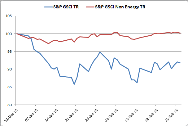
Ex-energy, commodities are positive for the year.  The S&P GSCI Non Energy Total Return is up 14 basis points in 2016, finally reaching a turning point after its near 20% loss in 2015. That is pretty good considering the -8.2% loss year-to-date for the S&P GSCI.

It is optimistic given tightening inventories in industrial metals, the weather hurting crop yields in agriculture and the sporadic but big oil gains. In particular, it might be most promising if oil rises since if oil rises, it helps all other commodities.

As of Feb. 26, 2015, the U.S. corporate bond market was valued at USD 8.3 trillion.[1]  For comparison, that’s larger than the GDP of Germany, France, and the U.K. combined.  Exhibit 1 details the growth of the U.S. corporate debt market since 2009, showing annual issuance amounts for both investment-grade and high-yield debt.  Since 2012, there has been USD 1.3 trillion[2] of U.S. high-yield corporate debt issued—more than the total amount issued in the prior 10-year period (2002-2011).

Given the low interest rate environment and the increased demand for yield, many U.S. corporations have taken advantage of the opportunity to borrow at lower costs.  What is interesting is how increased borrowing may not necessarily contribute to long-term growth.  Rather than investing in assets or technology, many companies used the proceeds from debt issuances to pay dividends or support buyback programs.  As evidence, dividends paid out by companies in the S&P 500^® in 2015 amounted to the highest proportion of their earnings since 2009.

Further, using the constituents of the S&P 500 Bond Index, measures of debt relative to cash flows are at levels not seen since 2008 (see Exhibit 2).

Also noteworthy is the amount of U.S. corporate debt that is scheduled to mature in the next five years.  Recent reports from rating agencies state that as much as USD 4 trillion[3] in U.S.-rated corporate debt is set to mature through 2020.

Of the USD 3.7 trillion of corporate debt tracked by the S&P 500 Bond Index, over USD 1.5 trillion (approximately 40%) is set to mature through 2020 (see Exhibit 3).

While the past six years have been conducive for corporate debt issuance, the current environment of easy monetary conditions may not continue.  As seen with the recent turmoil with high-yield debt, the market’s ability or willingness to support debt refinancing is not always present.  As credit concerns escalate, corporations may face the possibility of increased funding costs or limited refinancing options.

[1]   Source: SIFMA

[2]   Source: SIFMA

[3]   Source: Standard & Poor’s Ratings Services Credit Services Ratings & Research (RatingsDirect^®)

In spite of the complex and volatile global markets, the Mexican government issued bonds in the international market for the second time this year.  In January 2016, it issued USD 2.25 billion in bonds with a coupon of 4.125%, and on Feb. 16, 2016, it issued two other types of bonds denominated in euros, totaling € 2.5 billion, or approximately USD 2.8 billion.  All of this adds up to a total of USD 5 billion, which represents 80% of the foreign debt financial needs for 2016.

The new bonds issued in euros were issued with a yield close to historic minimums in the euro market.  The first was for € 1.5 billion, with a maturity in 2022, which was offered at a yield of 1.98% and a coupon of 1.875%.  The second was for € 1 billion, maturing in 2031 at a yield of 3.424%, with a coupon of 3.375%.  The demand had a ratio of 1.76, with more than 280 international investors.  According to the Ministry of Finance (Secretaría de Hacienda y Crédito Público), the level of participation showed the trust in public finances and the good management of public debt.  Also, it established new references to provide liquidity to the yield curve in euros.

Considering the bond issuances since 2010, Exhibit 1 illustrates the amount issued in U.S. dollars (taking into account bonds in U.S. dollars, euros, British pounds, and Japanese yen), divided by maturity.  We can see that 44% of the total (USD 20.75 billion) will mature between 2021 and 2030.  Exhibit 2 shows the amount issued by currency and that 61% of the total amount is issued in U.S. dollars.

S&P Dow Jones Indices seeks to track the bond issuances in U.S. dollars with a maturity of over one year with the S&P/Valmer Mexico Government International 1+ Year UMS Index.  Exhibit 3 shows the annual returns of the index for the past five years and the depreciation of the Mexican peso against the U.S. dollar.  We can see that annual high returns are correlated with a depreciation of the currency.

We’ve written at length of the many historical benefits of the low volatility anomaly. The S&P 500 Low Volatility Index selects the 100 least- volatile members of the S&P 500 index; lacking any sector constraints, the index seeks to provide pure exposure to the low volatility factor. In doing this, it has experienced a large tracking error (9.5%) relative to the S&P 500.

Some asset owners are not comfortable with such a large tracking error. While it would be easy to dismiss low vol on the grounds of tracking error, the decision need not be binary.   The chart below plots the tracking errors at various levels of exposure to the S&P 500 Low Volatility index. The remainder of the equity exposure in these points is to the S&P 500. For example, if 50% is allocated to Low Vol, the other 50% is allocated to the 500.

The key takeaway is that tracking error increases proportionally as low vol allocation is increased. Unsurprisingly, the benefit of exposure to low vol increases as allocation to low vol increases.

A fund comfortable with 4% tracking error may resist a 100% allocation to low vol but could still benefit from a 40% allocation.  Historically, that would have provided enhanced return with a reduction in volatility versus the S&P 500. When it comes to low vol, a little exposure goes a long way.

Okay, the mono-line insurance companies aren’t going to enjoy this note.  After all, yields of insured bonds should be lower than bonds that are un-insured.  Prior to the great recession approximately half of the municipal bonds outstanding were insured and during that time insured bonds were more in demand than un-insured bonds.  Beginning with the great recession we have seen yields of insured bonds higher than un-insured bonds as questions about the viability of the insurers themselves were prominent worries in the market place.  It is understood that not all mono-line insurers are the same credit quality, some are stronger than others.  However, in aggregate the impact is impressive.

Using the weighted average yields of bonds in the S&P Municipal Bond Insured Index and the S&P Municipal Bond Investment Grade Index the difference can be highlighted. The result has been yield ‘pickup’ between insured and investment grade municipal bonds as of Feb. 25 2016 was 28bps.  In general, it is cheaper to buy insured bonds than un-insured bonds and as a result returns have been higher.

Chart 1: Select municipal bond indices and their yields and returns over three year period

The risk of generalizing or over simplifying the complex municipal bond market  is inherent in any broad analysis.  Each issuer and each mono-line insurer has their own credit profile. The indices aggregate the bonds to provide the weighted average statistics used.