Get Indexology® Blog updates via email.

In This List

Who’s in charge of your investments – Captain Kirk or Mr. Spock?

Will Greece Default, And Does It Matter?

Questions and Answers from our Passive vs Active Webinar

The Fed’s Rate Increase Is Looking Like a Game of Kick the Can

Tax-Aware Australia: An Idea Whose TAIM Has Come?

Who’s in charge of your investments – Captain Kirk or Mr. Spock?

Contributor Image
Philip Murphy

Former Managing Director, Global Head of Index Governance

S&P Dow Jones Indices

I have a confession – earning the market return minus expenses does not feel very enticing. Reasonably well-run index funds will do just that, and probably land within the 2nd or 3rd performance quartile year in and year out. But is that the best I can do? Where’s the satisfaction? My inner Captain Kirk wants an investment that will crush the market.

On the other hand, my inner Spock guides me to observe empirical data and apply logic. And Mr. Spock is telling me that if I want to compound returns effectively over time, which is the only way I know of to grow wealth, indexing is my friend. Here’s why:

Look at the odds. In every period there are some active managers that outperform the market. But the chances of picking a manager that outperforms in the next period and into future periods are quite slim. Here’s a table showing results of active small-cap funds from our December 2014 issue of Persistence Scorecard:

Persistence Table

Almost 30% of 1st quartile small-cap funds, as of September 2011, had fallen to the 4th quartile as of September 2014. Only 22% repeated their 1st quartile performance. Random odds would give a 25% chance if funds did not close, merge, or liquidate. The persistence data shows that active small-cap managers tend to move about in terms of their relative standing. It’s quite likely that if one is fortunate enough to invest with a 1st quartile manager in one period, the manager may fall in performance rankings in future periods.

Do the arithmetic of compound returns. I downloaded 3-year annualized total returns, as of April 2015 based upon monthly data, of small-cap active and passive mutual fund share classes in the Morningstar database. My sample is not adjusted for survivorship, so active returns appear better than actual experience. I then created a hypothetical example showing the impact of investing $1000 and earning the median of 1st quartile returns (the 87.5th percentile) of active small-cap share classes for a 3-year period, and earning the median of 4th quartile returns (the 12.5th percentile) of active small-cap share classes for the following 3-year period. I compared this investment with another where I invested $1000 and earned the median 3-year annualized return (the 50th percentile) of all small-cap index fund share classes for six years. Here are the results of my hypothetical example:

Compound Growth

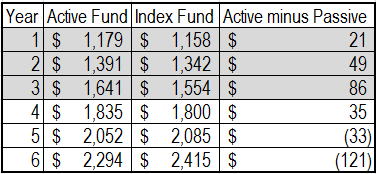
After three years, the active strategy is winning by $86. But by the fifth year the slow and steady median small-cap index fund is out in front by $33. After the sixth year, the active strategy is behind by $121. Maybe earning consistent 2nd – 3rd quartile returns is not so dull after all. In any event, I’m betting that maximizing my chances to “Live long and prosper…” will lead to more lifelong satisfaction than going for short term emotional gratification. Sorry Captain Kirk.

I’m presenting this material, along with some related ideas this Thursday afternoon during a complimentary webinar, “Not All Small-Cap Indices are Created Equal,” hosted by S&P DJI.

The posts on this blog are opinions, not advice. Please read our Disclaimers.

Will Greece Default, And Does It Matter?

Contributor Image
Tim Edwards

Managing Director, Index Investment Strategy

S&P Dow Jones Indices

Once again, Europe’s banking and finance chiefs are hunkered around the negotiating table. The Greek prime minister is optimistic a deal can be reached, the German finance minister dismissive. A debt payment is due; it is two minutes to midnight.  The markets are hanging by a thread on the outcome.

Writing the news is getting easy – just cut and paste from the last time a Greek payment was due.

You could be forgiven for assuming nothing has changed, and a deal should be expected in the final hours of the latest crisis. This is at least an empirical approach.

But there are important distinctions to be drawn between the current impasse and previous ones.  If Greek equities, Greek bonds and Greek GDP disappeared, it would certainly be a tragedy, but not of epic and globally destructive proportions.  And it is more likely that Greece will default precisely because it is now bearable.

It is bearable because the IMF and the European Central Bank now own pretty much every bond on which the Greek government can default.  There other holders, but not many of them. By now, each knows the risks.

It is bearable because, while Europe’s equity markets as a whole amount to EUR €10 trillion,  our broad-based equity index for the region, the S&P Greece BMI, comprises just 39 stocks with a combined free-float market capitalization of EUR €19.7 billion – about two one-thousandths of the former.

It is bearable because the GDP of Greece is now less than 1.5% of Europe’s – an amount otherwise sufficient to distinguish a great quarter of growth from a one of mild disappointment.

Of course, the risks of a Greek default have always been in the unknowable, the fall in confidence, the “contagion” —  the secondary consequences.  And it is in this respect that the world is different. Europe’s economy overall is growing again, and is more immune to shock.  The majority of the region’s banks have completed stress tests in 2014 that, unlike the 2011 equivalents, explicitly tested robustness in the event of a default by Greece’s government.  The financial markets have had ample time to prepare for downstream effects.  Most importantly,  the economies and markets viewed as most likely to suffer from contagion —  Ireland, Italy, Portugal and, to a lesser extent, Spain – are looking much healthier.  It is harder to see the next domino to fall.

In short, a Greek default looks more palatable today than at any point since this crisis began.  And that is important precisely because political forces are at the heart of negotiations.  If a default is more economically bearable, it is more politically feasible.

Europe does not want Greece to default, but it is a balance.  The scales are now differently tipped. The Greek government does not wish to default either. But they were elected to renegotiate the terms of the current bailout agreements, remain in the euro currency block and to “end austerity”.  If not all of those objectives can be achieved, they may well see the last objective as paramount.  If a last minute deal is found, our headline can be put back into storage to be ready for the next crisis.

Thus characterized: a Greek default might indeed occur, but only if it doesn’t really matter.

The posts on this blog are opinions, not advice. Please read our Disclaimers.

Questions and Answers from our Passive vs Active Webinar

Contributor Image
Shaun Wurzbach

Managing Director, Head of Commercial Group (North America)

S&P Dow Jones Indices

In the last post I wrote, I mentioned that I recently moderated a global webinar for financial advisors on the topic of S&P DJI research on passive vs active.  We received 20 questions during the course of this webinar.  I thought that it would be interesting to share some of those questions from advisors and the answers that our panelists provided.  The replay of the webinar is available if you missed it.

Question:  To what extent does using S&P DJI’s proprietary indices affect the outcome of the SPIVA studies?

Answer from Aye Soe, Global Head of Index Research & Design at S&P Dow Jones Indices:  That certainly does matter.  A great example of how much it can matter is in the U.S. Smallcap space.  In research we recently published, we found that the S&P SmallCap 600 outperformed the Russell 2000 Index by 172 bps per annum between 1994 and 2014.  This example shows the importance of benchmark selection.

Question:  How could the SPIVA results change if you stripped out the closet indexers and only looked at truly active managers?

Answer from Rick Ferri, Founder and Managing Partner of Portfolio Solutions: We did not attempt to define what a closet indexer was or separate those funds from other actively managed funds.

Answer from Aye Soe:  We use the University of Chicago’s Center for Research in Security Prices (CRSP) Survivorship Bias Free Mutual Fund Database.  Our goal is to provide an “apples to apples” comparison in size, style, and other characteristics to compare indices to mutual funds.  Active share and closet Indexing are topics which seem to be getting more analytical attention, but closet indexers is not a strong definition or classification that we have yet incorporated into our research.

Question:  Is “alpha” a myth? (Since by definition index funds can’t achieve positive alpha)

Answer from Aye Soe:  SPIVA and Persistence, when used together show how difficult “alpha” is to deliver and sustain.  So it isn’t a myth but it might be described as rare.

We did not have time to answer all the questions we received during the webinar.  I followed up with our three presenters and then personally emailed consolidated answers from our presenters to each person who sent in a question.  I want to conclude by emphasizing that all three of our presenters made the point (which is documented in our Persistence Scorecard research) that past delivery of alpha is no guarantee of future delivery.   Rick questioned whether taking the chance in selecting active managers is a good bet.  He showed data on the median of outperformance and the median of underperformance indicating a negative skew.  Here is one graph from Rick’s study that shows this skew:

Capture

The posts on this blog are opinions, not advice. Please read our Disclaimers.

The Fed’s Rate Increase Is Looking Like a Game of Kick the Can

Contributor Image
Kevin Horan

Former Director, Fixed Income Indices

S&P Dow Jones Indices

Continued lackluster U.S. economic activity right up until today’s slower personal consumption expenditures (PCE) report may have pushed rates lower during the last week of the month and into June’s start.  The yield of the S&P U.S. Investment Grade Corporate Bond Index moved lower by 8 bps during the last week of the month to close at 2.89%.  The May closing yield was still 6 bps higher than the April closing yield of2.83%.  The index fell 0.47% for the month, and returned 1.10% YTD.  With the move down in Treasury rates, corporate issuance continued at an active pace as new issue deals from Home Depot (USD 2.5 billion), PNC Bank (USD 3 billion), Time Warner (USD 2.1 billion), UBS (USD 3 billion), and many more were launched.

Vigorous issuance also occurred in the high-yield market, as ArcelorMittal (USD 1 billion), CommScope Tech (USD 2 billion), MarkWest Energy (USD 2.45 billion), and WellCare Health (USD 0.3 billion) all issued last week.  The yield of the S&P U.S. High Yield Corporate Bond Index closed May lower by 6 bps, at 6.11%, compared with 6.16% at the start of the month.  Year-to-date, the yield of the index is 73 bps tighter than the Dec. 31, 2014, yield of 6.84%.  The index returned 0.51% for the month and returned 4.8% YTD.  Outside of a slightly negative March (-0.19%), the high-yield index continues to provide positive monthly performance.  The continued “kick the can down the road” approach to the Fed’s rate hike may have caused yield-craving investors to bide their time in the sector.  High-yield bonds appear likely to return 5% in 2015, according to Martin Fridson, a veteran follower of the asset class and CIO of Lehmann Livian Fridson Advisors.[1]

In the shadow of the high-yield index’s YTD performance, the S&P/LSTA U.S. Leveraged Loan 100 Index returned 2.64% YTD.  For May, the index returned 0.05%.  Like the investment-grade and high-yield markets, issuance activity ramped up after the long Memorial Day weekend with 10 issuers tapping the market for a combined USD 8.72 billion.

After an increase of 11 bps in April 2015, the yield of the S&P/BGCantor Current 10 Year U.S. Treasury Bond Index continued its upward trend throughout most of May.  The 10-year U.S. Treasury Bond regained support during the last week of the month as yield came back down to 2.13% after being as high as 2.29% during the month.  Post month-end trading continues to move yields lower as the Fed’s preferred measure of inflation unexpectedly slowed in April (Core PCE year-over-year, 1.2% versus 1.3% prior).  Overall for the month, the S&P/BGCantor Current 10 Year U.S. Treasury Bond Index closed 9 bps wider than its start of 2.04%.  For the month, the return of the index was -0.62%, while YTD it returned 1.61%.

U.S. TIPS, as measured by the S&P U.S. TIPS Index, fell by 0.95% for May, as the YTD return closed out the month at 0.97%.  Like nominal Treasuries, the TIPS index gained 0.27% the last week of May to help offset some of the prior three weeks of losses.  The report of a slower PCE index makes it harder for the Fed to begin raising rates as inflation remains low.

Source: S&P Dow Jones Indices LLC.  Data as of May 29, 2015, leverage loan data as of May 31, 2015.


[1] The Street: High-Yield Bonds May Outperform Stocks in 2015 Despite Oil Price Fears, Jan. 16, 2015.

The posts on this blog are opinions, not advice. Please read our Disclaimers.

Tax-Aware Australia: An Idea Whose TAIM Has Come?

Contributor Image
Harry Chemay

Co-Founder & CEO

Clover.com.au

This is the first blog in a series on the evolution of Australia’s tax-aware investment management (TAIM) landscape.  

In 1999, a new method of calculating Capital Gains Tax (CGT) was introduced in Australia, with assets acquired after its commencement taxed on the basis of time held and type of taxpayer. Assets held for less than 12 months are subject to CGT on the full gain at the taxpayer’s individual rate of tax.  Assets held for longer than 12 months have CGT applied at a discount of between 0% and 50%, depending on the type of taxpayer.

Prior to 1987, Australian companies were taxed on corporate earnings, and from these after-tax profits, would pay dividends.  Those dividends were then taxed in the hands of recipient shareholders at marginal rates as high as 60%.  The combined effect was a tax rate on dividends that could, in certain cases, exceed 78%.

The introduction of dividend imputation in 1987 removed the double taxation of dividends, with tax-resident Australian companies receiving a ‘franking credit’ for tax paid at prevailing corporate tax rates. Shareholders could then use these credits to offset tax on their dividends.  The imputation system was introduced to ensure that taxpayers in effect only paid ‘top up’ tax on dividends, being the difference between the corporate rate and the shareholder’s higher tax rate.

Under the original dividend imputation system, a shareholder with a lower tax rate than the prevailing corporate rate effectively received no value for the franking credits attached to their dividends. For Australia’s superannuation funds this was highly material.  In 1988, a tax rate of 15% had been introduced on the taxable income (including legislated employer contributions) of these pension vehicles.  Among the nation’s largest institutional investors, super funds could not take advantage of the ‘excess’ franking credits they were receiving.  This situation was remedied in 2000 when the tax laws were amended to allow excess franking credits to be claimed by low rate (and tax exempt) taxpayers.

To learn more about how to weigh your after-tax benefits, visit www.spdji.com/tax-aware.

The posts on this blog are opinions, not advice. Please read our Disclaimers.