


There are no conclusive definitions of an asset class or definitive lists of asset classes, but asset allocation depends on how one chooses to define asset classes that collectively form the opportunity set. A company owned by Morningstar called Ibbotson Associates together with PIMCO pulled together some research on the topic that I think is interesting. They present a framework based on three super asset classes:
1. Capital assets, such as stocks, bonds and real estate, provide an ongoing source of value that can be measured using the present value of future cash flows technique.
2. Consumable or transformable assets, like commodities, only provide a single cash flow.
3. Store of value assets such as currency and fine art are not consumed and do not generate income but do have a monetary value.
The identification of the investable opportunity set significantly changes the potential risk and return possibilities. In another model, asset classes can also be thought of as risk factors or market exposures that produce a return that is not based on skill. These market exposures include sensitivities to financial markets, interest rates, credit spreads, volatility and other market-related forces.
Commodities offer an inherent or natural return that is not conditional on skill. Coupled with the fact that commodities are the basic ingredients that build society, commodities are a unique asset class and should be treated as such. Together, their sources of return have provided an important portfolio function.
The component of return called expectational variance that is caused by unexpected inflation – or supply shocks- is the main driver of the return differences between commodities and also between commodities and other asset classes. It is typical to observe this in the low correlations between commodity sectors as shown in the table below.

However, there is an important distinction between the commodities “to be grown” and commodities “in the ground”. The commodities in the ground are energy and metals and are finite, while the agriculture and livestock are commodities “to be grown” and are able to be replenished. As David Jacks points out, since 1950, there is a major historical performance difference of real prices for “commodities in the ground” that rose by roughly 180% versus real prices for “commodities to be grown” that fell by roughly 33%. 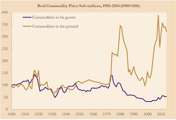
Source: http://apebc.ca/resources/Jacks_2015.pptx
This can be due to the scarcity factor of commodities “in the ground” but rather than a constant premium for scarcity, Jacks observes that typically, cycles in commodities “to be grown” are preceded by those “in the ground”. This time may be different from the transition of fixed capital accumulation to a consumption-based economy and suburbanization, but relies on the success of the CPC (Communist Party of China.) If the suburbanization is successful then we may see an increase in demand for goods “to be grown” and an inflection in long-run trend and we may also observe below-trend prices for goods “in the ground” and formation of new cycle in medium run.
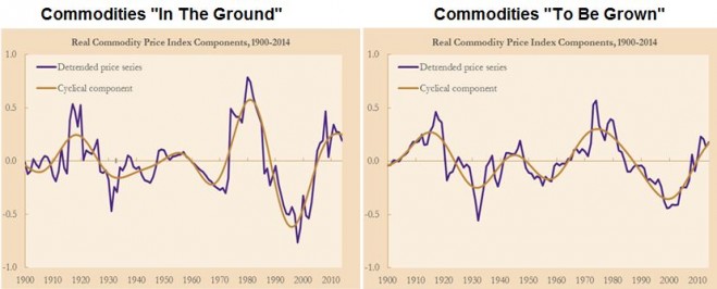
It is difficult to see these long-term cycles since the shorter term trends in place are noisy, particularly for the “to be grown” commodities. The prices are sensitive to immediate inventories driven by the balance of the individual supply and demand models where supply is impacted by the planting decisions, weather patterns, crop disease and technology that determine the crop yields from season to season.
For example, below is the chart of the one-year index levels of the S&P GSCI Energy & Metals versus the S&P GSCI Agriculture & Livestock:
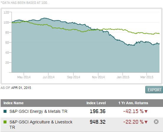
Yesterday, the USDA (U.S. Department of Agriculture) released Prospective Plantings report, one of its most important reports of the year. Soybeans in the index rose 57 basis points but corn and wheat fell 4.6% and 3.4%, respectively, after farmers were seen cutting their corn plantings by 500k acres less than expected even as supplies grow to highest levels in nearly 20 years. Today, corn and wheat rebounded, gaining 1.5% and 3.1%, respectively while soybeans continued to rise 1.7%. The next factors that may impact the crops are short term weather patterns and conditions that impact crop yield.
However, when thinking of long-term investing, it is important not to miss the forest for the trees and remember the asset class is providing diversification and inflation protection through time. Long-term investors like pensions may be able to use the points in the cycle rather than the short term trends to identify true opportunities that may help meet long-term liabilities.
The posts on this blog are opinions, not advice. Please read our Disclaimers.


