Indexology^® Blog

The uncertainty of the future of Puerto Rico municipal bonds continues to weigh on the municipal bond market. Bonds in the S&P Municipal Bond Puerto Rico Index have settled into an average price of just over 50 cents on the dollar with the low point of 47.27 on July 8^th 2014.   The index tracks over $73billion in par amount of bonds. Puerto Rico is an important segment of the municipal bond market as many of these federal and state tax-free bonds are held in State based mutual funds. While revenue bonds have held their own, year to date the S&P Municipal Bond Puerto Rico General Obligation Index has returned a negative 1.53%.

The uncertainty of how New Jersey will handle its financial future has resonated with the bond market. While Illinois gets a lot of press it is New Jersey general obligation bonds that are moving more like Puerto Rico bonds in 2015. The S&P Municipal Bond New Jersey General Obligation Index has seen its weighted average yield rise by 21bps in 2015 eerily similar to the rise of yields in the S&P Municipal Bond Puerto Rico General Obligation Index which have moved 22bps higher. The comparison is unfair of course. The weighted average yield of the S&P Municipal Bond New Jersey General Obligation Index ended at 1.73% up from 1.52%. The yields of bonds in the S&P Municipal Bond Puerto Rico General Obligation Index ended at 8.16%. Meanwhile, the yield of the S&P Municipal Bond New York General Obligation Index has dropped by 6bps to 1.43% and the yield of the S&P Municipal Bond Illinois General Obligation Index also has shown an improvement of 3bps to end at 2.74%.

Yields and Total Returns of Select State Municipal Bond Indices

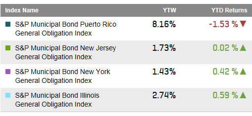
Source: S&P Dow Jones Indices LLC.  Data as of February 20, 2015.

The overall medical trend rates covering all services have continued to be modest in the S&P data through the 3^rd quarter of 2014—increasing up to 3.5% on a 12-month moving average basis as of September[1].

But the winter of 2014 was particularly harsh in much of the country and likely dampened utilization.  Late fall 2014 weather was cold and snowy, and recent weather in early February 2015 has become more severe.  If the severe weather reaches the equivalent level of 2014, there will likely be minimal impact on trends, since the effect in two successive years is likely to balance out, although regional impacts can vary with the weather differences by region between the two years.

Influenza results for the 2014-2015 season appear to be similar but possibly slightly less than the 2012-2013 season and higher than the 2013-2014 season based on several measures.  During the 2012-2013 season overall trends remained in the low single digits.  Charts A and B below show several years of history for outpatient flu visits (Chart A) and pneumonia and influenza mortality (Chart B) from the Centers for Disease Control and Prevention.

[1] We track the LG/ASO trends as representative of underlying trends, since Individual and Small Group are impacted more significantly by the Affordable Care Act (ACA).  Keep in mind that actual trends experienced by plans are likely to be higher than as reported in S&P data.  Trends experienced by large employers on plans that have not changed in the previous year could be higher by as much as 2% or more on bronze level plans and higher by 1% or more on gold level plans due to the effects of deductible and copay leverage.  So risk takers need to take this into account.  In addition, the S&P Indices do not reflect the impact of benefit buy-downs by employers (i.e., higher deductibles, etc.), since the indices are based on full allowed charges.  As noted above, actual trends experienced by employers and insurers in the absence of benefit buy-downs can be expected to be higher than reported S&P trends due to plan design issues such as deductibles, copays, out-of-pocket maximums, etc.   Benefit buy-downs do not represent trend changes since they are benefit reductions in exchange for premium concessions, but they can have a dampening effect on utilization due to higher member copayments, and this can have a dampening effect on measured S&P trends compared to plans with no benefit changes, further pushing up experienced trends relative to those reported in the indices.

THE REPORT IS PROVIDED “AS-IS” AND, TO THE MAXIMUM EXTENT PERMITTED BY APPLICABLE LAW, MILLIMAN DISCLAIMS ALL GUARANTEES AND WARRANTIES, WHETHER EXPRESS, IMPLIED OR STATUTORY, REGARDING THE REPORT, INCLUDING ANY WARRANTY OF FITNESS FOR A PARTICULAR PURPOSE, TITLE, MERCHANTABILITY, AND NON-INFRINGEMENT.

Having touched a low of 1.66% as of mid-February 2015, the yield of the S&P/BGCantor Current 10 Year U.S. Treasury Index bounced up to close at 2.05% on Feb. 13, 2015. The move away from the safety of Treasuries came as an impasse occurred in the negotiations between Greece and their EMU partners. European officials continue to wrestle over terms for a plan to support Greece, which could run out of money as soon as the end of March. If a deal cannot be struck, then the fear of European contagion could cause a move back down in yield for U.S. Treasuries.
For now, the focus of the markets may be circling back to the Fed and the possibility of a rate increase as soon as this June. The improving U.S. economy should naturally lead to higher rates, in order to match the economic growth. Such a policy change would move rates higher to the front-end of the curve, leaving the longer-end to represent investor outlook and reactions. The open-ended question is what other political, market, or global forces could curtail rising rates.

The S&P U.S. Aggregate Bond Index is up 0.78% YTD, though the rise in yields for February has translated to a loss of -1.10% MTD. The investment-grade corporate component of the aggregate index, as measured by the S&P U.S. Investment Grade Corporate Bond Index, is 29% of the parent index, and has contributed 1.09% of total return YTD, while also providing -1.44% return MTD. The only larger component of the aggregate index is the S&P/BGCantor U.S. Treasury Bond Index (38% of the parent index), which has returned 0.62% YTD, while losing 1.43% MTD.
Lower-rated credit indices such as the S&P U.S. High Yield Corporate Bond Index and the S&P/LSTA U.S. Leveraged Loan 100 Index have not greatly outpaced investment grade corporates YTD, given the increase in risks. For the month of February, however, they have performed well, as Treasury rates have been increasing. The high-yield index has returned 1.70% YTD and 1.19% for February. Likewise, the S&P/LSTA U.S. Leveraged Loan 100 Index has returned 1.11% YTD and 0.91% MTD.

What happens to other commodities when oil prices spike? On one hand, if oil rises so much that an economic slowdown overpowers the tax-break effect, then commodities might fall. However, oil is a main input to produce many other commodities so prices of goods can rise when oil prices increase. The latter scenario is more likely given the historical relationship of energy to inflation and to other commodities.

One of the hallmarks of diversification in commodities is how lowly correlated they are to each other from the individual supply and demand models.  Notice the highest correlation between any two sectors in the chart below is 0.27.

The source of return that mainly drives the correlation between commodities to be unrelated is expectational variance or supply shocks.  When oil price falls, it may be demand or supply driven but most of the time the weakness has come from demand drops. When this happens, the correlation is higher between commodities at about 0.40 on average. However, the recent moves (both down and up) have been more driven by supply than demand, as the case has been in many historical oil price spikes.

This can be observed with the lower correlation of about 0.2 between oil and other commodities during oil price spikes, but despite the lower correlation, all commodities rise with rising oil.  A supply driven oil bull is the best because it pulls other commodities up with it but with very low correlation, a measure of lockstep but not magnitude.

Since the concept of  a strong upward force on commodities as oil prices rise but with low correlation can be difficult to explain and understand, below is a quick correlation refresher with a few hypothetical and real illustrations.

For example, both of these charts below show a perfect correlation of +1.0. However, the top chart on average has a down month of -1.0% for each oil and gold. The bottom chart has an average down month for oil of -1.0% but while oil is down gold only drops on average 25 basis points.

The next hypothetical chart shows zero correlation but a directional pull.  Both oil and gold are always up. Oil is up 1% every month on average while gold is up 4.6% on average. They are always both up at the same time but there is little control of lockstep despite a directional relationship.

Below is an actual example between WTI (blue) and unleaded gasoline (yellow) where the magnitude of average increases are almost exact, yet the correlation is only 0.6. Out of 66 positive WTI oil months in the past 10 years, there were only 10 months where unleaded gas dropped, showing it is difficult for gas to fall when oil rises.

Let’s pick copper as a different example. It has very low correlation of 0.18 to oil when oil is rising. However, it on average had a monthly return of 3.85% when oil was positive and returned positive in 71% or in 47/66 of those months. Copper generally was pulled up with oil, just at various magnitudes, making the correlation low.

Below are some highlights of commodity relationships to oil as oil prices rise and fall.

Fed watchers will study the FOMC minutes for hints of the next interest rate move.  However, the most important data – the January employment report – was published more than a week after the FOMC meeting. That report showed strong job growth not just in January but over the last few months as data revisions presented a clearer picture of the economy.  Many Fed watchers seem to be discounting the Employment Report and focusing on low oil prices and declines in the consumer and producer price indices.  Recent comments by FOMC members suggest that the era of the zero Fed funds rate could end as soon as June, only four months away.

With the unemployment rate at 5.7%, weekly initial unemployment claims running at about 300 thousand per week and payrolls expanding consistently there is no doubt that the economy is enjoying strong growth.  The inflation picture is more debatable.  The Core CPI – excluding food and energy – is up about 1.5% over the last 12 months and is close enough to the Fed’s 2% goal to support returning interest rates to normal (non-zero) levels.  Oil is a question. The price of WTI crude oil made a recent low of $44.45 on January 28^th but has now advanced to $52.60 on February 17^th. No one knows what oil will do next or when it might rebound to the over-$100 level of last June. However, many US oil producers cannot sustain their business at current prices. There is a growing sense that, sooner or later, oil prices will rise, even if they don’t return to triple digits. When oil prices do rise, they will echo through the economy and boost other prices as well. Both the employment strength and concerns about a possible rebound in oil prices argue for an increase in the Fed funds rate.

Comments from FOMC members since the last meeting in late January point to an early move on interest rates.  The data are cited as evidence that the economy is strong and that risks are shifting to more inflation rather than more unemployment. Among those suggesting an early shift to more normal interest rates are Jeffrey Lacker of the Richmond Fed, John Williams of the San Francisco Fed, Loretta Mester of the Cleveland Fed and Esther George of the Kansas City Fed.   The FOMC vote count  may be more interesting than usual in the last, and next, set of minutes.

Many Fed watchers are expecting, or arguing for, continuing the current policy of close to zero interest rates.  While agreeing that the US economy seems strong for the moment, they fear secular stagnation – the idea that potential US economic growth is capped at around 2%, less than the 2.5% to 4% experienced in recent decades.  Potential GDP growth can be gauged by the sum of labor force growth plus productivity. Among developed nations the US is one of the few where population is growing, although growth is slowing and the population is aging pointing for slower labor force growth.  Recent labor force growth is under one percent and productivity is about three-quarters of one percent giving potential GDP growth of 1.75%.  The argument is that if potential growth is this low, now is not the time to slow down the economy or dampen employment gains.

The FOMC members may be more concerned with near term risks that economic strength could run into rebounding oil prices and raise inflation expectations.  And the members are the people who make the rate decisions.

The FOMC minutes will be released at about 2 PM on Wednesday February 18th