Indexology^® Blog

Markets are down over 20%, COVID-19 is a global pandemic, negative global growth is looming—all of that just in the first 20 days of March! During same time period, VIX rose 65%, while the S&P 500 VIX Short-Term Futures Index jumped 175%. With a long-term beta of 0.7 to spot, a question might be—why did the S&P 500 VIX Short-Term Futures Index jump more than the spot?

The reason for this is that March was a time for catching up. In February, the spot jumped 113%, while the front two months’ futures lagged, rising 44% and 30%, respectively, thereby leading to a 134% and 146% respective catch-up in March.

Now, interestingly, the S&P 500 VIX Short-Term Futures Index, an unleveraged hypothetical basket of the first two VIX futures contracts, returned more than either of its constituents. This is because of “roll yield” due to the curve being in backwardation—where rolling an expensive first month to a cheaper second month adds to returns. VIX has been backwardated since Feb. 24, 2020, as shown in an earlier blog.

Exhibit 1 shows the VIX term structure on Jan. 2, 2020 (in contango) and on March 20, 2020 (in backwardation). In the first case, the S&P 500 VIX Short-Term Futures Index sold first-month futures at USD 14.08 and bought the same second month portion at USD 16.13, incurring a per-unit roll cost of USD 2.05. While on March 20, 2020, the daily roll of the index would sell higher at USD 61.53 and buy lower at USD 56.63, thus enjoying a per-unit profit of USD 4.90. Since VIX futures were backwardated for almost a month, this additional roll return was not negligible.

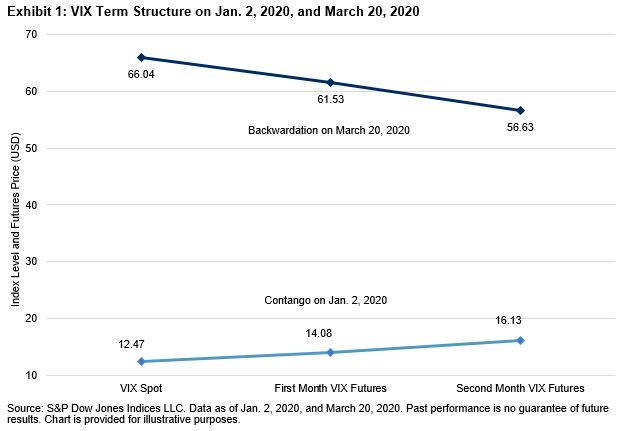
If a VIX futures gradient on a given day is quantified as its slope between the first- and second-month contracts, a positive slope (or a contango) amounts to a roll cost, while a negative slope (or backwardation) yields a roll carry.

Further, we define monthly average VIX futures gradient as the average of daily slopes during that month. Since the S&P 500 VIX Short-Term Futures Index rolls continuously, this is essentially the actual monthly roll cost. A positive number indicates cost, while a negative number indicates roll yield. Exhibit 2 shows that the daily roll in the first 20 days of March contributed a positive return of 13% to the index return.

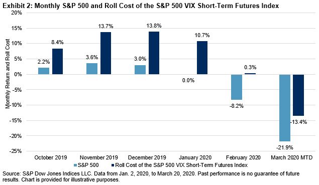
Exhibit 3 shows that the negative correlation between the S&P 500 VIX Short-Term Futures Index and the S&P 500 is stronger in a bear market than in a bull market. Interestingly, the correlation between its monthly roll cost and the equities market is also much stronger when the market goes down (see Exhibit 4). Thus, in a stressed market, it is more likely that the VIX futures term structure will be backwardated and investors will benefit from the daily roll of the index.

Vladimir Lenin said, “There are decades where nothing happens; and there are weeks where decades happen.” While the market has faced unprecedented pressure from a pandemic, the S&P 500 VIX Short-Term Futures Index has generated positive returns from the elevated VIX level and the roll yield from the VIX futures term structure. Backwardation is uncommon, but it has come to the rescue when it was needed most.

The S&P Balanced Global Bond and Equity Futures Index (the S&P BEF Index) is designed to deliver consistent returns through various market cycles by exploiting the complementarity between equities and bonds during market crisis, and adjusting the allocation to component indices on a daily basis to achieve a stable risk level (what we call a dynamic volatility control mechanism). The components are rolled futures that are highly liquid and tradable, and are as follows.

• Equities Basket: The S&P-500 (SPX), Euro STOXX 50 (SXSE), and Nikkei 225 (NKY) Rolling Futures.
• Bond Basket: U.S. Treasuries, Euro Bund, and JGB Notes Rolling Futures.

Over the past 20 years, S&P BEF 0.4% Decrement Index[1] posted an annualized return of 3.84%, a risk-adjusted return of 1.13, and a maximum drawdown of 5.55% (see Exhibit 1).

How did the index perform during historical crises?

The S&P BEF 0.4% Decrement Index posted positive returns of 2.7% during the Dot-Com Bubble Crisis and 3.6% during the Eurozone Crisis. This is in stark contrast to the significant losses posted by the S&P 500^® during those periods.

Throughout the 2008 Global Financial Crisis (GFC), the S&P BEF 0.4% Decrement Index declined 2.3%, while S&P 500 lost 50% during the same period. The index recovered rather quickly within six months compared with the four years that the S&P 500 took. The S&P BEF Index’s asset allocation around the GFC is shown in Exhibit 3.

1. When the crisis began in August 2007, the leverage ratio was swiftly reduced from the high point of 140% to 120% by mainly cutting equity exposure by 20%.
2. As the market was affected by escalated volatility, equity exposure was further reduced to 11% in March 2008.
3. Before the bankruptcy of Lehman Brothers in September 2008, the S&P BEF Index switched to “minimum investment” mode, with merely 2.5% allocation in equities and 46% in bonds. Until February 2009, equity exposure was limited to 5%.
4. In the recovery period, as volatility decreased, the leverage ratio gradually returned back to 113% with 95% in bonds and 18% in equities in September 2009.

How has the index performed so far in 2020?

As of March 16, the S&P BEF 0.4% Decrement Index declined 1.5% YTD and was off 3.7% since February 19. In comparison, the S&P 500 plunged by 26% and 29.5%, respectively.

Similar to what happened in the GFC, the S&P BEF Index first reacted to the increasing volatility in the stock market by cutting its equity allocation from 40% on January 15 to 20% on February 28, while maintaining the bond allocation at its maximum of 100% (see Exhibit 4). During this period, bond market soared and the strategy benefited from that.

After oil prices crashed and COVID-19 was escalated to a pandemic, Treasuries started to fall on March 9 as well. To tackle the widespread volatility, the S&P BEF Index turned on “minimum investment” mode by significantly reducing allocations to both equity and bond baskets. As of March 16, 2020, the index had only 5.4% equity exposure and 63.8% bond exposure. The leverage would further decrease if the market situation worsened.

What is special about the current market environment is that the levels of volatility varied among major regions, potentially because of the different phases of virus spread. Throughout January, we saw greater volatility in Europe and Japan than in the U.S. And during this period, the index assigned an average allocation of 17.3% to S&P 500 futures, greater than the 11.5% allocated to the Euro Stoxx 50 and the 9.2% allocated to the Nikkei 225 (see Exhibit 5). By March 16, allocation to the three regional equity indices changed to 1.8% for S&P 500, 1.4% for Euro Stoxx 50, and 2.2% for Nikkei 225. Likewise, when a certain market’s volatility starts to come down, the risk control mechanism will be able to dial up the allocation to that specific region in the future.

The S&P BEF Index aims to deliver higher long-term risk-adjusted returns with a smoother wealth curve than a single asset might. Historically, it rode through the Dot-Com Bubble, 2008 GFC, and Eurozone Crisis. In 2020, the S&P BEF Index has worked well so far.

[1] The S&P BEF 0.4% Decrement Index tracks the S&P BEF Index less a fixed fee of 0.4% per year.

Have the new beta-like ESG indices delivered on their objectives, notwithstanding the market turmoil? The answer is yes, and then some. The S&P 500^® ESG Index has provided low tracking error relative to the S&P 500 and similar risk, but also a better return.

For decades, growth in ESG investing was unremarkable, held back by investors’ fears that they were inviting underperformance relative to the market by integrating their values into their investments. However, in 2019, assets in ESG funds suddenly spiked. In ETFs alone, assets increased from USD 22.1 to USD 56.8 billion.[1] What brought this about? The launch of popular new indices, like the S&P 500 ESG Index, which were built to maintain overall industry group weights characteristics similar to those of their underlying benchmarks.

These beta-like indices gave investors’ comfort that they could integrate ESG into the core of their portfolios. Was this warm feeling deserved? As Exhibit 1 shows, the ESG versions of the S&P 500, S&P Europe 350^®, S&P Global LargeMidCap, and S&P Developed LargeMidCap indices all performed better than their beta counterparts. The only major category in which the ESG version underperformed was emerging markets.

Because these indices are new, however, it is important to acknowledge that three- and five-year return figures include history that was built before these indices launched in early 2019, as noted in the methodology. For this reason, investors should pay special attention to the past year or so, when the indices were live. As Exhibit 2 highlights, the ESG indices have posted low returns, in line with the market, but the ESG versions have mostly outperformed beta, with the S&P 500 ESG Index beating the S&P 500 by 100 bps YTD. Again, only the S&P Emerging Market LargeMidCap ESG Index underperformed its beta peer.

What produced these results? Simply put, it was how the index methodology sorted the largest companies that drove performance.

To recap our standard ESG index methodology, it was designed to retain most companies in the benchmark index, weighting those that remain by market capitalization. Companies are excluded only if they: (a) have a low ESG score relative to their industry peers; (b) are involved in controversial weapons or tobacco production or sales; (c) are not closely adhering to the UN Global Compact; or (d) are involved in severe controversies.

Because the index is market capitalization weighted, the ESG index methodology has to properly sift the largest companies for the ESG benchmark to perform in line with its objective. In this respect, the 2019 rebalance seems to have largely been on the mark. Some companies that were significant drivers of the S&P 500’s performance in the past 12 months, such as Apple and Microsoft, passed through the screens and remained in the S&P 500 ESG Index. Other major companies with less-than-stellar performance, such as Boeing, were excluded.[2]

Will the S&P 500 ESG Index continue to track and even improve on the performance of the S&P 500 in the future? Common sense and our lawyers prevent us from speculating, but it appears that the ESG indices are passing major tests—their first year live, their first rebalance, and their first bout with market volatility—even better than expected.

[1] Source: S&P Dow Jones Indices.

[2] Boeing was excluded from the S&P 500 ESG Index because of its involvement in controversial weapons.

The week ending March 20, 2020, marked one of the worst weeks for the Indian equities market, with the S&P BSE SENSEX witnessing record lows. The index recovered 5% to close at 29,915 (price return [PR]) on Friday, March 20, 2020, but it was still 17% down as compared with the week before, when it was at 34,103 (PR) on March 13, 2020. Historically, the last time the S&P BSE SENSEX witnessed such large fluctuations was on May 18, 2009, when the index gained 2,110 in a single day, increasing 17.34%.

The effect of the coronavirus has transformed global and local markets, as well as their behavior. We are witnessing a similar pattern in equities markets across the world, be it the S&P 500^® in the U.S., the S&P BSE SENSEX in India, the S&P/ASX 200 in Australia, the S&P Japan 500 in Japan, or the S&P Europe 350®. Fig 1 shows the trends from February 29, 2020, to March 20, 2020.

A comparison below reflect the trend for a month and Fig 2 reflects how they have performed over longer periods in comparison to the recent short-term trend.

Fig 1 – Global Indices Movement this month

Source: S&P Dow Jones Indices LLC. Data from February 29, 2020, to March 20, 2020. Past performance is no guarantee of future results. Chart and table are provided for illustrative purposes.

Fig 2 – Comparison of Global Indices

Source: S&P Dow Jones Indices LLC. Past performance is no guarantee of future results. Chart and table are provided for illustrative purposes.

Market volatility has always been a challenge, and while traders and investors could benefit from it in some markets, in other markets, appropriate strategies are available for managing this in investment portfolios. Low volatility, though an anomaly, is a strategy that works ideally in highly volatile situations.[1] We see this phenomenon across countries, and India is no different.

The S&P BSE Low Volatility Index posted a month-to-date total return of -13.96% versus the S&P BSE SENSEX’s total return of -21.72% as of March 19, 2020 (see Fig 3). If we compare the trend over longer periods, the low volatility strategy shows a similar result (see Exhibit 3). The aim of this strategy is to participate on the upside while protecting on the downside. The S&P BSE Low Volatility Index is designed to track the performance of the 30 companies in the S&P BSE LargeMidCap with the lowest volatilities, as measured by standard deviation.

Fig 3 – Movement of the Indian Indices this month

Source: S&P Dow Jones Indices LLC. Past performance is no guarantee of future results. Chart and table are provided for illustrative purposes.

Fig 4 – Performance of the S&P BSE Low Volatility Index

Source: S&P Dow Jones Indices LLC. Past performance is no guarantee of future results. Chart and table are provided for illustrative purposes.

[1] https://spindices.com/indexology/factors/is-the-low-volatility-anomaly-universal

In January 2019, we highlighted several indices designed to reduce the impact of large equity market drawdowns. Here we analyze the same suite of indices divided across three broad categories: defensive equity, multi-asset, and volatility. This analysis simply reviews performance since the S&P 500®’s high on Feb. 19, 2020, through the close on Friday, March 20, 2020.[1]

The current bear market has progressed with extraordinary rapidity—there have been only 22 trading days since the S&P 500 reached its all-time high. As such, any conclusion we draw must be considered strictly preliminary. Moreover, it’s important to begin any evaluation with a reasonable set of expectations. Defensive equity indices are, after all, still equities; we hope that they will mitigate losses in the underlying benchmarks, but they’ll still go down, perhaps substantially. Loss mitigation should increase in multi-asset indices, which are able to shift capital away from a declining equity market. Finally, indices that can take a long position in volatility might, at least in the current circumstances, be the best risk mitigators of all.

Defensive Equity

This category includes three well-known index series: the S&P Low Volatility Indices, S&P Quality Indices, and S&P Dividend Aristocrats^® Indices. These indices have attracted significant inflows, particularly in recent years, as investors have balanced their need to maintain a position in equities with concerns about an aging bull market. As of the close on Friday, March 20, 2020, two of the three were beating their benchmark, the S&P 500, despite having just come through an extraordinarily difficult week. Coming into last week, the S&P 500 Low Volatility Index had recorded meaningful outperformance but then had a particularly tough week due to overweight positions in Real Estate and Utilities, two of the hardest hit sectors.

Multi-Asset

Multi-asset indices combine imperfectly-correlated asset classes (such as stocks and bonds) with the goal of creating broadly diversified portfolios. These indices employ disciplined asset allocation rules and dynamically adjust their leverage or allocation with the aim of achieving a more stable risk profile.

As expected, many of these indices have de-leveraged or increased allocations to safe-haven assets as volatility has increased in recent weeks. Thus far, several have posted double-digit drawdowns, which is not surprising when almost all asset classes are down. However, losses have been muted and many of our indices have posted meaningful outperformance compared to equities.

Volatility

Volatility can be thought of as an asset class in its own right, which market participants can use to access uncorrelated returns, provide downside protection, and improve risk-adjusted performance. Indices in this category either invest directly in volatility or use it as an allocation signal.

As you will see in Exhibit 3, the Cboe S&P 500 Buffer Protect Index Balanced Series posted meaningful outperformance. This is due to the fact that each monthly index within this series “buffer protects” against the first 10% of losses in the S&P 500 over a set period of time. The S&P 500 Dynamic VEQTOR Index, which rebalanced in and out of cash and increased its allocation to short-term VIX^® futures as the VIX spiked, recorded positive returns, up 7.9%.

[1] For more details on these individual indices, please see: Seeking Volatility Protection Using Indices.