Indexology^® Blog

If there were dreams to sell, a poet asked, what would you buy?  Much more prosaically, if you could design your dream investment process, what would it look like?

A simple way to think about the question is to separate success into two dimensions: frequency and magnitude.  Frequency means how often we “win” (i.e., how often our strategy outperforms its benchmark); magnitude measures the size of the winnings (i.e., the average value added when we win, and the average value lost when we lose).  In the best of all possible worlds, we’d win most of the time, and the average outperformance in our winning months would be much higher than the average underperformance in our losing months.

Since we don’t live in the best of all possible worlds, compromise is necessary.  Suppose we could only outperform half the time.  Our investment process would still be a net winner if its wins were bigger than its losses — in other words, if its average outperformance (during winning months) were bigger than its average underperformance (during losing months).

Dispersion gives us a way to gauge the likely differences between the returns of a particular strategy and those of a market benchmark.  This is true whether the strategy in question is active or is a factor or “smart beta” index.  When dispersion is high, the strategy is likely to deviate from its benchmark by a relatively large amount; when dispersion is low, deviations are likely to be smaller.  So: if our wins occur when dispersion is relatively high, and our losses when dispersion is relatively low — our investment process might still accumulate considerable value, even it wins only half the time.

There’s a strong historical tendency for high dispersion and negative returns to go hand-in-hand, as shown here for the S&P 500:

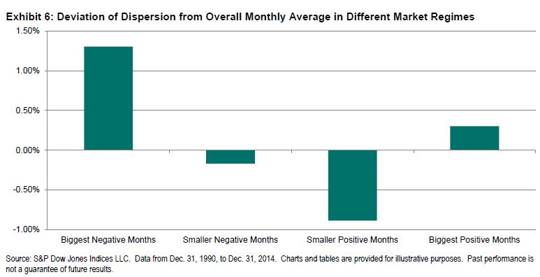
When the S&P 500’s returns are at their most negative, dispersion tends to be well above average.  When returns are positive, dispersion tends to be slightly below average.  This means, other things equal, that a strategy that tends to win when the market is down and to lose when the market is up will have a natural performance advantage, since its hits will occur in times of high dispersion.

This is exactly the pattern of returns exhibited by low volatility indices, as well as by other defensive strategies such as the S&P 500 Dividend Aristocrats.  We expect such strategies to do relatively well when the market declines.  The remarkable thing about them is that they also tend to outperform over the long run, despite the market’s secular upward bias.  Arguably, this is because they tend to win when dispersion is relatively high, and to lose when dispersion is relatively low.  They are therefore more likely to outperform when the reward for outperformance is high.

Differential returns can often be a consequence of index dispersion.  The distribution of dispersion favors strategies that outperform in down markets.

This is the second in a series of blog posts relating to the in depth analysis of performance differential between the S&P SmallCap 600 and the Russell 2000.

Numerous studies have been conducted on Russell’s annual reconstitution process in June, particularly regarding the downward price pressure placed on the Russell 2000.  As winners from the Russell 2000 move up to the Russell 1000, and losers from the Russell 1000 move down to the small-cap index, small-cap fund managers are forced to sell winners and buy losers, thereby creating negative momentum.

To study this effect, we examine the average monthly excess returns for each calendar month from 1994 through 2014.  It is seen that the S&P SmallCap 600 has an average monthly excess return of +0.68% for the month of July vs. the Russell 2000, with a statistically significant t-stat of 2.54.  These results indicate that there may be a strong relationship between the Russell 2000 annual rebalancing in June and the negative excess returns in the following month.

In an attempt to control for the July reconstitution effect, a hypothetical index was created where the monthly returns are represented by the Russell 2000, with the exception of July being represented by the S&P SmallCap 600.  From 1994 through 2014, the difference in an investment of USD 1.00 into each the Russell 2000 and the S&P SmallCap 600 amounts to USD 2.41 (USD 6.18 and USD 8.59 respectively).  The same investment in the hypothetical index results in USD 7.17, USD 1.42 lower than the S&P SmallCap 600.  Therefore, only a portion of the excess returns may be attributed to the July reconstitution effect, with the rest of the difference coming from other factors.

Although the low volatility anomaly was first documented more than 40 years ago, it was the trepidation and volatility in the years following the most recent financial crisis that propelled the concept to the forefront of investor interest.  In recent years, the phenomenon has been well covered, by both academics and the investment community, in the form of innovative financial instruments that exploit the anomaly and subsequent attraction of assets to those vehicles.  The low volatility anomaly exists not just in the U.S., but instead seems to be universal.  The current debate is less focused on the existence of a low volatility effect and more on the construction of various strategies to exploit the phenomenon.

In the U.S., for example, the S&P 500^® Low Volatility Index outperformed its benchmark, the S&P 500, from 1991 to 2014 by 101 bps compounded annually—with 31% less volatility.  What is the reason for its success?  Our rankings-based method of portfolio construction not only screens for stocks by factor, it also weights by factor (or the inverse of the factor, in this case) to achieve its objective.  This methodology has resulted in large sector weights, historically.

However, strategic sector tilts don’t paint the complete picture here.  If we only apply the returns of the S&P 500 sectors to the respective sector weights in S&P 500 Low Volatility Index over the last 24 years, the “hypothetical” low volatility portfolio can account for 69% of the total risk reduction.  This means that being in the “correct” sector during this period accounted for more than two-thirds of the volatility reduction achieved by the S&P 500 Low Volatility Index (see Exhibit 1).  In the same period, the return increment attributed to being in the “correct” sector was only 29%, from which we can conclude that more than two-thirds of the outperformance is idiosyncratic to S&P 500 Low Volatility Index’s methodology.

As is the case with many factor-driven portfolios, various portfolio construction methods can result in lower volatility.  The ability to protect the portfolio in relatively stable sectors is a feature—not a side effect—of the S&P 500 Low Volatility Index’s rankings-based methodology.

Oil price shocks and a revisit of deflationary concerns in Europe are just some of the “gifts” the New Year has brought in 2015 to increase volatility in global financial markets.  The concern for financial advisors is that loss of invested capital may come with volatility if there is a need or a client decision to sell.  For those U.S.-based financial advisors already skeptical about the strength and stamina of the U.S. equity bull market, some now perceive a fork in the road.  They can continue down the path of diversification, or they can explore a path of adopting more proactive and potentially more costly risk management as a means of preventing loss.

Whether a financial advisor needs to do more than adequately diversify client portfolios is a subject of debate within the advisor community.  At the emotional heart of the debate is the question, “How much can your clients bear to lose?”

Some financial advisors have a “memory” from the last recession that diversification, or asset allocation failed.  How strong that memory of failure is may depend on how heavily their portfolio was tilted to U.S. large-cap equities or other risky assets during the time of the recession.  Citing data and analysis from Sam Stovall, U.S. Equity Strategist at S&P Capital IQ:

The Bear Market Price percentage decline of the S&P 500® in 2007-2009 was much worse than average at -57% (Sam found the average price decline of the S&P 500 during Bear Markets to be -38%, going back to September 1929)

• Every sector of the S&P 500 experienced a decline in 2007-2009
• Isolating 2008, nearly all asset classes experienced declines; with the Barclay’s Aggregate (+5.2%) and Long Treasuries (+24.0%) being two notable exceptions

Importantly, and seemingly in contrast to a view that diversification “failed,” Sam found that a 60/40 portfolio (S&P 500/Long Term Treasury Bonds) returned -12.6% over this same period of time in 2007-2009.  While this piece of Sam’s data and analysis is from a very thorough presentation,  Sam has said that “…maybe it is our memory that failed us and not diversification.”  Or it could be that even a loss of 12.6% is too much loss for some financial advisors.

Regardless of perceptions of the success or failure of diversification, some asset managers and advisors who are portfolio managers take the view that diversification may not be sufficient for their clients’ needs to prevent loss of capital in times like the recession of 2007-2009.  I recently asked Jerry Miccolis, Principal and Chief Investment Officer of Giralda Advisors to discuss asset allocation and portfolio risk management and his analysis, testing, and modeling of a number of index benchmarks based on S&P DJI and CBOE indices.  I invite you to read our entire interview with him.  For those short on time, Jerry told me that diversification is not sufficient for his clients’ needs because it will not guarantee “…sufficient risk management in times of severe market stress.”  Jerry points out that during such times, it is possible for correlations among asset classes to rise and that the Great Recession provided a recent example of that.

Financial advisors and the asset managers who serve them can’t tell precisely when the next Great Recession will come.  They have to decide in advance whether asset allocation is sufficient or whether they will follow a path of more aggressive risk management.  Since proactive risk management comes at a cost, a tool which might help financial advisors to determine the value of risk management beyond diversification is appropriate benchmarks for risk-managed portfolios.

Having announced that the European Central Bank will stimulate its economy though additional purchases, bonds had seen demand recently. Now all eyes are on the U.S. employment data. The markets were quiet going into the release of the employment number as investors waited with some anticipation for direction. Activity did pick up as the U.S. number reported positive economic news that non-farm payrolls were up 25% more than expected. (Estimate: 235K jobs, actual: 295K).

During this week, the 10-year reference bond increase 19bps (5.63% to 5.82%), causing the S&P/Valmer Mexico Government MBONOS Index to lose 1.07% (64.16% annualized). After today’s NFP release, the yield-to-maturity of the 10-year is 5.96%, 14bps up from the previous close and the spread to Treasuries widened to 373 bps.

Real rates also moved significantly this week increasing 17bps causing the S&P/Valmer Mexico Government Inflation-Linked UDIBONOS Index to lose 1.42% (85.24% annualized). February’s CPI will be public next Monday (March 9^th), it’s expected to be a 3.01% annual, less than the 3.07% for January.

The Mexican peso has depreciated since the start of the month by 1.47%, from 14.95 to last nights close of 15.17.  Today the currency is up 1.97% (15.47).  Continued currency depreciation of the peso means that the strength of the U.S. Dollar has helped the return of the S&P/Valmer Mexico Government International UMS Index to be less of a loss at -2.48% annualized.