Get Indexology® Blog updates via email.

In This List

Dividend Payers Outperform Non-Dividend Payers in Colombia

The Case for Dividend Futures Contracts

Uncertainty’s Curse on Confidence

Accessing Energy and Energy Infrastructure through Master Limited Partnerships (MLPs)

Iron Ore Is on a Hot Roll

Dividend Payers Outperform Non-Dividend Payers in Colombia

Contributor Image
Cristopher Anguiano

Senior Analyst, U.S. Equity Indices

S&P Dow Jones Indices

In a previous blog,[1] we explored historical dividend payers in the Colombian equity market, focusing on the S&P Colombia BMI as the underlying universe, highlighting the number of dividend payers, market capitalization, and GICS® sector distribution. Building on that, we now examine if the Colombian market has rewarded dividend payers over non-payers.

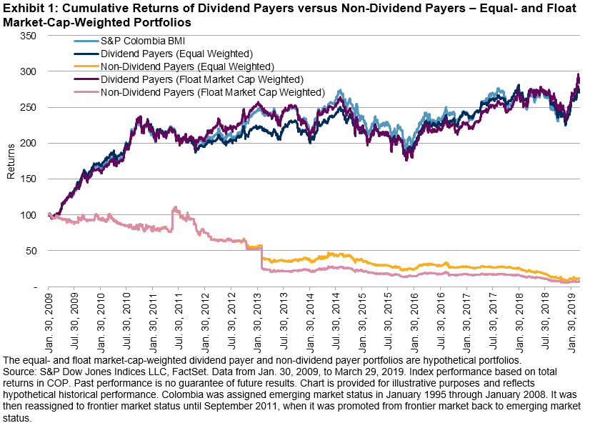
As a starting point, we formed hypothetical portfolios by grouping the underlying universe into dividend payers and non-dividend payers. Portfolios are float market cap weighted as well as equal weighted to remove any size bias. Each portfolio rebalances semiannually in March and September. The 10-year back-tested performance shows that both equal-weighted and float market-cap-weighted dividend payer portfolios outperformed non-dividend payers on a cumulative basis (see Exhibit 1).

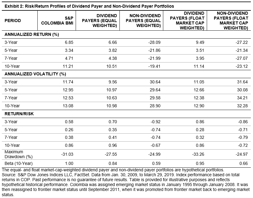
The risk/return profiles of the hypothetical portfolios (see Exhibit 2) reveal that the dividend payer portfolios outperformed the non-dividend payer portfolios on a risk-adjusted basis. It is worth noting that the realized volatilities of the dividend payer portfolios were lower than the broad market as well as the non-dividend payer portfolios, for equal-weighted and float market-cap-weighted versions. The betas of the dividend payer portfolios were higher than those of non-dividend payers, coming in close to one. Therefore, the dividend payer portfolios were more sensitive to the market.

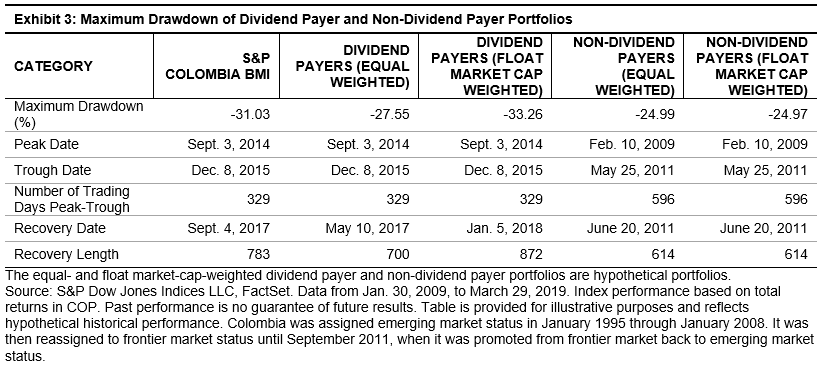
Similarly, dividend payer portfolios had higher maximum drawdowns than non-dividend payer portfolios. Exhibit 3 shows that the largest drawdowns for non-dividend payer portfolios were similar for both weighting methods. Although the dividend payer portfolios’ peak and trough dates were in line with the market, maximum drawdowns and recovery lengths were larger for capitalization-weighted portfolios.

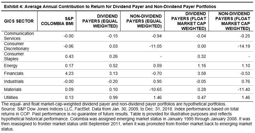
Next, we looked at the average annual contribution to return over the 10-year period, broken down by sectors (see Exhibit 4). We can see that dividend payer portfolios followed a similar distribution to that of the underlying universe, with Financials being the largest contributor, followed by Utilities and Energy. This result is consistent with our previous blog, where we highlighted that these sectors were the largest contributors to dividend yield. For the Energy sector, which contains only one security, the free-float portfolio contribution was larger than the equal-weighted version.

For the non-dividend payer portfolios, Consumer Discretionary and Materials were the biggest detractors. Financials slightly underperformed and Industrials issues outperformed their dividend payer counterparts, while Consumer Staples had zero contribution, as all the Consumer Staples securities pay dividends. The Utilities and Energy sectors also added positively for all the portfolios, while Communication Services contributed negatively to all portfolios.

Overall, the Colombian equity market has seemed to prefer dividend payers to non-dividend payers. This finding implies that dividend-based strategies are feasible, but market participants may want to address potential sector concentration issues.

[1]   https://www.indexologyblog.com/2019/05/22/examining-dividend-payers-in-colombia/

The posts on this blog are opinions, not advice. Please read our Disclaimers.

The Case for Dividend Futures Contracts

Contributor Image
Tianyin Cheng

Former Senior Director, ESG Indices

S&P Dow Jones Indices

The S&P 500® Dividend Points Index tracks dividend payments of S&P 500 constituents, based on a fixed initial market capitalization, independent of equity price changes. The index cannot be invested in directly, but it is tracked by futures contracts listed on the Chicago Mercantile Exchange (CME). Currently, the annual dividend futures are available up to 10 years forward.

The S&P 500 Dividend Points Index represents cumulative cash dividends paid over a defined period of either one quarter or one year. At the start of the next period, the index is reset to zero so that it reflects dividends paid in discrete periods that coincide with the expiration of S&P 500 futures.

Dividend Futures Use Cases

One important use case of dividend futures (and the OTC swap markets that emerged prior to the futures markets) is dividend risk hedging in structured equity products sold by investment banks, which have been popular in Europe and some Asian countries, such as Korea and Japan.

These products offer equity-linked returns to end clients, although the payouts are usually linked to price changes rather than total returns in the underlying equity index. If a bank hedges with an index futures or basket of equities, they are left with exposure to dividends, which has significant implication on hedging risk.

The dividend futures market enables banks to reduce some of their dividend exposure by selling dividend futures to sophisticated investors. The supply of dividends and the corresponding low demand results in low implied future dividend growth and attracts hedge funds to the dividend market, adding further liquidity and increasing the appeal of dividend transactions. Asset owners may also be willing to buy dividend futures in order to hedge out dividend fluctuation risk in order to better match their liability streams.

How Dividend Futures Work

If a long position in the dividend futures contract is held to expiration, the investment return depends on the difference between the index dividends per share actually paid on the S&P 500 and the price of the dividend futures at the time of the initial investment. The dividend futures price should reflect the market’s best guess as to what the fair value of the future dividends will be, although short-term supply and demand will cause prices to fluctuate around fair value.

According to the dividend discount model, the intrinsic value of a stock equates to the present value of a stock’s future dividends. Therefore, dividend futures prices would generally benefit from stock price increases, especially when looking at a long horizon. In addition, dividend payments tend to be fairly well estimated close to a year before they are paid. Therefore, as the futures get closer to expiry, the futures price sensitivity to stock price decreases (see Exhibit 1).

Dividend Futures versus Estimated Dividend

As of May 31, 2019, the December 2029 S&P 500 Annual Dividend Futures contract priced to 67.4 versus 57.9 for the 2019 contract. This implies a modest 1.5% annualized dividend growth rate over the next 10 years (see Exhibit 2). This growth rate is much lower when compared with the 6% annual dividend growth rate from the past 49 years (from 1970 to 2018).

When we compare the dividend futures prices with forecasted dividends, we can also see a clear gap. The dark blue bar in Exhibit 3 reflects the current dividend futures price; the yellow bars reflect the analyst consensus estimate.

Both the historical dividend growth trend and the dividend estimates seem to indicate that dividend futures are undervalued and may have a 4%-5% upside annually for a buy and hold strategy. One explanation for this “dividend premium” is that banks’ activity creates natural sellers of dividend futures, with a resulting potential return for buyers. Another explanation is the perceived risk of negative dividend surprises. In that sense, the return is simply compensation for risk.

Exhibit 4 demonstrates a buy and hold strategy for the front year dividend futures contract—it longs the next annual dividend futures contract for a year, and when the contract expires, it rolls into the next year’s contract. Such a strategy returned 2.6% per year with a volatility of 2.3% from Dec. 18, 2015, to May 31, 2019.

The posts on this blog are opinions, not advice. Please read our Disclaimers.

Uncertainty’s Curse on Confidence

Contributor Image
Stuart Magrath

Former Senior Director, Channel Management, Australia and New Zealand

S&P Dow Jones Indices

With the dust still settling after the unexpected result of Australia’s recent federal election on May 18, 2019, which resulted in a third 3-year term for the incumbent Liberal-National Party coalition, the Australian government has quickly turned its attention to a slowing in the Australian economy.

While the uncertainty over franking credit refunds and negative gearing on investment properties is over, and despite a recent fillip in residential auction clearance rates, Australia’s unbroken record of 27 recession-free years may still be in danger of being derailed by offshore events. In addition to a keen focus on economic matters, expectations are that the government will quickly turn its focus to legislating the majority of the recommendations from the Royal Commission into Misconduct in the Banking, Superannuation, and Financial Services Industry once the Governor-General opens the 46th Parliament in early July 2019.

For this reason, financial advisers in Australia will likely continue to grapple with major disruption in their industry in 2019 and for the next few years to come. Adding to the Royal Commission outfall, the Financial Adviser Standards and Ethics Authority (FASEA) requirements are now in place for advisers, with the education standards having to be met prior to Jan. 1, 2024.

Despite all these headwinds, many opportunities remain for advisers to transform their practices, and index-based investment solutions could be a vital part of that transformation. We recently published our semiannual Australian Persistence Year-End 2018 Scorecard, and once again, we saw that relatively few active funds were able to stay on top over time. With the results of the SPIVA® Australia Year-End 2018 Scorecard, we can continue to say with confidence that most active managers underperform most of the time.

The latest Australian Persistence Scorecard measured the performance persistence of active funds that outperformed their peers and benchmarks over consecutive three- and five-year periods, and analyzed their transition to other quartiles over subsequent periods. Overall results suggested that only a minority of high-performing funds persisted in outperforming their respective benchmarks, or consistently stayed in their respective top quartiles, over consecutive three- and five-year periods. Among top-quartile funds across all asset classes, 9.7% and 2.2% consistently maintained top-quartile rankings over the consecutive three- and five-year periods, respectively. Top-quartile funds in the Australian Bonds fund category had the lowest turnover over both periods.

With this data, financial advisers could recommend index-linked investment solutions to their clients, explaining that it is difficult to select an active fund that will outperform its relevant benchmark, and that it would be even more difficult to select an active fund that will do so consistently.

The posts on this blog are opinions, not advice. Please read our Disclaimers.

Accessing Energy and Energy Infrastructure through Master Limited Partnerships (MLPs)

Contributor Image
Qing Li

Director, Global Research & Design

S&P Dow Jones Indices

In 2018, the U.S. set world production records for both natural gas and oil.[1] The growth in production is expected to continue and the U.S. is set to become a net energy exporter[2] by 2020, ending a 75-year period of dependence on imports.

The increase in energy production not only shifts the dynamics of the global oil market, but also increases the demand for strong energy infrastructure to support the processing, transporting, and storage of oil and gas. An average of USD 14.7 billion in capital expenditures for a pipeline of oil, gas, and natural gas liquids would be needed from now through 2035 to support this demand.[3]

In addition to providing exposure to energy and energy infrastructure, MLPs provide a tax advantage[4] and stable income. The latter is due to MLPs distributing the majority of their earnings in cash. Using the S&P MLP Index to represent the asset class, our analysis shows that MLPs offer potential diversification benefits. Based on monthly return data from August 2001 to April 2019, MLPs showed low or negative correlations with traditional asset classes such as stocks and bonds (see Exhibit 1).[5]

Historically, MLPs demonstrated solid performance in various market environments. The S&P MLP Index outperformed the overall stock market in 10 out of 18 years (see Exhibit 2) and outperformed the bond market in all market environments with an average excess return of 0.5%. This is higher than the excess returns from Utilities (0.29%), Energy (0.36%), and the broad equity market (0.31%; see Exhibit 3). Owing to a positive outlook on the Energy sector and its infrastructure, the S&P MLP Index gained 17.57% YTD in 2019 (as of April 2019).

Using 18 years of index history, we can see that MLPs had attractive yield, with an average annual dividend yield of 6.6%, compared with 1.9% from equities, and 2.2% and 3.4% from the Energy and Utilities sectors, respectively (see Exhibit 4). Although the recent tax reform[6] may make MLPs less attractive than they used to be, the taxable income from MLPs continues be subject to single-level taxation.

In general, MLPs can not only provide exposure to the Energy sector, they also stand to gain from the increase in demand for energy infrastructure and higher yield.

[1]   U.S. Energy Information Administration (EIA), March 14, 2019 and April 15, 2019.

[2]   Annual Energy Outlook 2019, EIA, Jan. 24, 2019.

[3]   North American Midstream Infrastructure through 2035, the INGAA Foundation, Inc., June 18, 2018.

[4]   Being set up as a pass-through entity, an MLP allows all the gains and losses to flow through to the individual partners (unitholder) directly and the business entity does not need to pay income tax.

[5]   We use the S&P MLP Index, S&P 500, and Bloomberg Barclays U.S. Aggregate Bond Index to represent MLPs, stocks, and bonds, respectively.

[6]   The Tax Cuts and Jobs Act of 2017 cut corporate tax from 35% to 21%.

The posts on this blog are opinions, not advice. Please read our Disclaimers.

Iron Ore Is on a Hot Roll

Contributor Image
Jim Wiederhold

Former Director, Commodities and Real Assets

S&P Dow Jones Indices

The S&P GSCI Iron Ore has been on a tear this year, up 72.47% YTD as of June 13, 2019, breaking through the previous high from May 22, 2019. It had by far the best YTD performance out of any of the commodities indices in the S&P GSCI Series. This bullish performance during the first half of 2019 is a good example of how using commodities in a tactical way can boost returns for investors. The S&P GSCI Iron Ore was able to distance itself from other metals. For example, the S&P GSCI Industrial Metals was flat over the same period.

Prior to the recent rally, the S&P GSCI Iron Ore was relatively range bound for two years due to competing macro themes. There are several factors to point to when explaining the recent YTD performance. First, the challenging risk-off environment in Q4 2018 left most assets finishing the year in the red. This allowed for neutral-to-bearish investor positioning entering 2019, especially for those commodities with a high beta to global markets and specifically to Chinese economic activity.

Second, to ease the burden of U.S. tariffs and to support the slowing economy, Beijing announced a variety of stimulus measures focused on boosting its industrial complex. China currently purchases approximately two-thirds of seaborne iron ore. As has been seen in the last few years with each China hard landing or global growth scare, the People’s Bank of China has not hesitated to turn on its most-adored stimulus levers. Those levers have historically been ways to increase funding for construction and infrastructure projects. While the planned move away from manufacturing to a more consumer-based economy continues to creep along in China, it will likely take a long time to implement this plan, and the Chinese administration appreciates that the current most effective way to support economic growth remains via these industrial support levers. The S&P GSCI Iron Ore is highly correlated to Chinese economic indicators such as real estate investment, industrial production, and steel production. Several of these indicators spiked in Q1 2019 just as iron ore prices started to rise (see Exhibit 2). It is worth noting that the most recent industrial production number dropped to a five-year low of 5%.

Third and most important, supply has been drastically curtailed in recent months. Inventories held globally have been reduced and are on pace to fall to five-year lows within the next few months. The Vale dam collapse in Brazil in late January 2019 and a cyclone in Australia in March 2019 reduced supply from the world’s two largest iron ore exporters. Shipments from Australia have largely returned to normal, but it is likely that Brazilian iron ore exports will be constrained for an extended period of time. Imported iron ore stock at Chinese ports fell to a 2.5 year low of 121.6mm metric tons in mid-June 2019 according to Steelhome.

The iron ore market has a number of characteristics that make it distinctive as an investable asset, but these characteristics are relatively common among commodities; iron ore supply is concentrated in a handful of geographic regions and controlled by a small number of players, and demand is dictated by one major end-user (China). Both supply and demand are subject to shocks caused by geopolitical events, unforeseen natural disasters, and policy decisions, as well as the actions of individual asset owners. However, with unique characteristics can come unique tactical investment opportunities for investors.

The posts on this blog are opinions, not advice. Please read our Disclaimers.