Indexology^® Blog

The S&P/ASX Australian Index Series has played a significant role in characterizing the Australian equity market performance since its inception in April 2000. Since then, the S&P/ASX 200 has served as the foundation for benchmarks and index-based investing strategies from sectors to quality, value, and momentum factor approaches.

Following the launch of the S&P 500^® ESG Index, which uses the new S&P DJI ESG Scores,[1] S&P Dow Jones Indices is proud to announce the launch of the S&P/ASX 200 ESG Index.

In this blog, we will focus on the role the S&P/ASX 200 ESG Index provides as the ESG alternative to mainstream listed equities investing in the Australian market. Using the new S&P DJI ESG Scores and other ESG data to define the index’s eligible universe, the S&P/ASX 200 ESG Index targets 75% of the market capitalization of each GICS^® industry group in the S&P/ASX 200. The outcome is to provide an improved index ESG score relative to the benchmark, while providing similar risk and returns, allowing investors to easily put their investment beliefs into action.

The S&P ESG Indices target an improved ESG index profile by allocating to the best 75% of the GICS industry group market capitalization in each benchmark’s eligible universe by ESG score rank. The index’s eligible universe is defined as all benchmark constituents after the removal of companies:

• with specific involvement in the production or sales of tobacco or controversial weapons or low levels of compliance with the principles of the UN Global Compact or
• in the lowest 25% of S&P DJI ESG scores among their global GICS industry group peers.[2]

The remaining constituents find themselves market-capitalization-weighted in an index that has historically closely tracked its benchmark, while yielding an improved ESG profile. These indices are designed for investors wishing to integrate ESG factors into their investments without straying far from the benchmark’s risk and return profiles (see Exhibit 2), making them an appealing alternative to core domestic and global allocations.

Additional Resources on the S&P ESG Index Series

• FAQs: S&P ESG Index Series
• Steadman, Reid, and Perrone, Daniel. “The S&P 500^® ESG Index: Integrating Environmental, Social, and Governance Values into the Core.” S&P Dow Jones Indices. April 2019
• The S&P ESG Index Series Methodology

[1]   The S&P DJI ESG Scores are based on data gathered by SAM, a division of RobecoSAM, through SAM’s Corporate Sustainability Assessment (CSA).

[2]   The index also accounts for ESG controversies that arise in its companies via SAM’s Media and Stakeholder Analysis (MSA), which continually monitors media for potential ESG-related events that could challenge the ESG scores SAM had assigned to companies.

Notwithstanding the recent correction associated with renewed trade tensions between the U.S. and China, a strong start to the year for global equity and commodities markets suggests a strong macroeconomic backdrop and a high risk appetite among investors. However, when drilling down into the performance of individual commodities sectors, it is clear that the situation is much more nuanced.

The global commodities market has been dominated by the strength of the petroleum complex so far this year; the intensity of oil supply disruptions has largely overwhelmed middling oil demand and the seemingly perpetual expansion of U.S. oil production, pushing Brent oil prices back up toward USD 75/barrel, albeit briefly. Oil supply constraints have varied from voluntary OPEC production cuts, to rising tensions among various actors in the Middle East, to U.S. sanctions on Venezuela and Iran. While additional supply disruptions are always a risk in the oil market, it is becoming more difficult to see where new disruptions may occur, and fading economic growth prospects in emerging markets as well as the trade conflict between the U.S and China could put increasing pressure on oil consumption growth and energy prices.

Meanwhile, the recent retracement in industrial metals prices reflects the rekindling of the trade war between the U.S. and China. Metals such as aluminium, nickel, and copper are used extensively in the production of goods targeted by U.S. tariffs, such as electronics. More broadly, higher tariffs also add to the existing headwinds facing the Chinese economy, although it is important to remember that Chinese authorities have the capacity to initiate significant economic stimulus should they deem the impact of the trade war too onerous for specific industries or too detrimental to the prospects for broad economic growth.

While investor and central bank interest in gold remains well above that of previous years, the performance of the gold market has been meek, which is rather at odds with the more cautious view of the world economy presented by recent weakness in the oil and metals markets. That said, there are growing signals coming from various central banks that monetary policy may become more accommodative in the second half of the year in response to flattering prospects for global economic growth, which is likely to support gold prices.

The agriculture sector has been a drain on the performance of the overall commodities market during the first five months of 2019. Agriculture markets are not generally dependent on the macroeconomic environment, but a number of agricultural commodities, such as soybeans, have also been drawn into the U.S.-China trade fracas. The spread of African swine fever, which will cut demand for pig feed, and bumper harvests in North and South America have also contributed to soybean prices falling to a post-financial crisis low.

The latter part of the global economic cycle is typically characterized by the outperformance of industrial commodities, namely energy and industrial metals. While commodities are not anticipatory assets, they can provide a useful insight into current macroeconomic conditions on top of any commodities-specific supply and demand dynamic. It is imperative that investors take stock of the myriad of indicators presented by commodities markets, especially given growing economic and geopolitical turbulence.

The Narendra Modi government will soon complete its five years in power. With polling underway to elect the next government, India is in election mode. Everyone is discussing politics and predicting the election results. The backers of the current government claim that the return of Modi will provide stability and ensure development. On the other hand, those backing the opposition, the Congress-led United Progressive Alliance, claim that a change in government is required in order to maintain secular harmony in the country. Neither side would welcome a hung parliament.

Over the past five years, the government made several landmark policy decisions and initiatives like the Goods and Services Tax (GST), demonetization, Insolvency and Bankruptcy Code, and Real Estate (Regulation and Development) Act, among others. Many of the reforms have had a major impact on the Indian economy. Even after disruptive reforms like the demonetization and GST, economic growth is back on track. Opinion surveys conducted before the polling suggest a close fight and the current government may not achieve the majority it got last time. The outcome is anyone’s guess until the counting begins on May 23, 2019.

The S&P BSE SENSEX TR moved from 30,242.22 on April 30, 2014, to 56,443.02 on April 30, 2019—a five-year absolute return of 86.64%. The S&P BSE AllCap, a broad benchmark index with over 1,000 constituents, had a five-year absolute return of 94.49%. Among the size indices, the five-year absolute return of the S&P BSE MidCap was the highest, at 115.35%, followed by the S&P BSE SmallCap, at 103.98%, while the S&P BSE LargeCap was at 86.70%. Exhibit 1 depicts the total returns of the S&P BSE SENSEX, S&P BSE AllCap, S&P BSE LargeCap, S&P BSE MidCap, and S&P BSE SmallCap for the five-year period ending on April 30, 2019. The capital markets in India have presented significant returns to investors in the past five years.

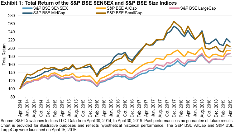
Exhibit 2 provides the five-year absolute returns of the S&P BSE AllCap Series. Among the sub-sector indices in the S&P BSE AllCap, the S&P BSE Finance and the S&P BSE Energy posted the best five-year absolute returns of 133.40% and 130.81%, respectively, while the S&P BSE Telecom had the worst return, at -15.92%.

Source: S&P Dow Jones Indices LLC. Data from April 30, 2014, to April 30, 2019. Past performance is no guarantee of future results. Table is provided for illustrative purposes and reflects hypothetical historical performance. The S&P BSE AllCap, S&P BSE LargeCap, S&P BSE Finance, S&P BSE Energy, S&P BSE Consumer Discretionary Goods & Services, S&P BSE Basic Materials, S&P BSE Utilities, S&P BSE Industrials, and S&P BSE Telecom were launched on April 15, 2015.

Market gains in the first four months in 2019 more than made up for what it lost in the turbulent last quarter of 2018 as the S&P 500 jumped 18%. Predictably enough, the S&P 500 Low Volatility Index^® trailed the broader benchmark (up a “mere” 16% in the first four months), although Low Vol has led the broader benchmark during May’s pullback.

The May rebalance (effective at the close on May 17^th) yielded minimal change in the sector distribution within the low volatility index. The most significant changes include added allocations to Financials and a scaling back of Technology.

Financials Became More Significant as Health Care and Technology Scaled Back in the Latest Rebalance for the S&P 500 Low Volatility Index

Trailing one-year volatility for each S&P 500 sector declined in the last three months. The volatility reduction was more or less equally distributed, so it’s not surprising that the latest rebalance wrought minimal changes in sector exposure for Low Vol. In fact, this latest rebalance is notable for its low turnover. The index replaced only 9 names, nearly half the count of the average of 17 over the last two years.

252-Day Volatility Declined Across All S&P 500 Sectors Compared to Three Months Ago

Global equities have been turbulent recently as a combination of stalled trade negotiations and announcements of tit-for-tat tariffs increased the prospect of a trade war between the U.S. and China.  After its historic start to the year, the S&P 500 is down 3.7% so far in May, while many other markets have also faltered month-to-date.  Amid the recent market jitters, many investors may be interested in strategies that help navigate periods of heightened volatility.

Many index-based strategies are designed to ride out turbulent times.  Among the most popular defensive equity strategies are low volatility and minimum volatility indices.  However, while both strategies are based on the low volatility anomaly and have similar names and objectives, they are constructed differently.  Low volatility indices rank constituents by their trailing volatility and select the least volatile stocks, whereas minimum volatility indices use an optimization-based approach to construct the least volatile portfolio.  Hence, low volatility indices comprise only low volatility stocks, whereas minimum volatility indices may contain highly volatile stocks.  Exhibit 1 shows the differences in portfolio construction for the S&P 500 Low Volatility Index and the S&P 500 Minimum Volatility Index.

Exhibit 1: Low & Minimum Volatility Indices are constructed differentlySource:  “Inside Low Volatility Indices”.  Table is provided for illustrative purposes.

Exhibit 2 shows that the differences in methodologies impacted the indices’ risk/return profiles: the S&P 500 Low Volatility has offered greater downside protection – and higher risk-adjusted returns – than its minimum volatility counterpart since December 1990.  Indeed, the low volatility index typically captured less than half of S&P 500’s total return in “down” months (determined by whether the S&P 500 posted a monthly decline), compared to around 70% for the minimum volatility index.

Exhibit 2: Low & Minimum Volatility Indices Behaved Differently

Another difference between low and minimum volatility indices is their geographic revenue exposure: around 80% of the S&P 500 Low Volatility’s revenues come from the U.S, compared to 66% for the S&P 500 Minimum Volatility.  Exhibit 3 helps to explain this result; it shows the sector exposures (height of the bars) and the domestic revenue exposures (bar labels) of companies within each sector for each index.  Clearly, the low volatility index has sizable allocations to more domestically-focused companies, especially within the Utilities, Real Estate, and Financials sectors.  On the other hand, the S&P 500 Minimum Volatility has greater exposure to companies that are more reliant on revenues from abroad.

Exhibit 3:  Low & Minimum Volatility indices may have different revenue exposures

As a result, while low and minimum volatility strategies have similar sounding names and objectives, they can behave differently over time.  Combined with differences in sectoral allocations and geographic revenue exposures, and how this may impact performance in the event of an escalation of trade tensions, market participants may be well served to take a deeper look inside low volatility indices.