Get Indexology® Blog updates via email.

In This List

Evolving From Single-Factor to Multifactor Investing

Commodities Are Like a Box of Chocolates, if You Only Factor in Interest Rates and the U.S. Dollar

The Rise of Sectors: Active and Passive Applications

Low Volatility Effect in the U.S. Preferred Stock Market

How Much Will My Retirement Income Cost? Part 2

Evolving From Single-Factor to Multifactor Investing

Contributor Image
Akash Jain

Director, Global Research & Design

S&P BSE Indices

This article is the third in a series of blogs. The previous two were titled “Factor Investing 101” and “How Do Single Factors Perform in Different Market Regimes in India?” This blog discusses sectoral tilts of different single factors and  varying correlations between factors in different market cycles.

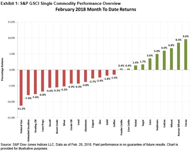
In our report, sector bias typically existed in factor portfolios, and differentials on sector exposure across factor portfolios were strongly associated with the unique cyclical nature of factor performance. Exhibit 1 highlights the two most overweight and most underweight sectors, on average, for each factor over the period from March 2006 to March 2017. Value and dividend were overweight in basic materials, whereas momentum, quality, and size were overweight in consumer discretionary goods & services. The finance sector was most underrepresented in the momentum, quality, low volatility, and size portfolios, and the information technology sector was underweight in value, dividend, and size portfolios.

Exhibit 1: Sector Bias Versus the S&P BSE LargeMidCap
FACTOR Most Overweight Sectors and Weight Differential (%) Versus Benchmark Most Underweight Sectors and Weight Differential (%) Versus Benchmark
Value Basic Materials, 13.7 Information Technology, -10.9
Energy, 7.7 Fast Moving Consumer Goods, -8.1
Momentum Healthcare, 6.2 Finance, -6.0
Consumer Discretionary
Goods & Services, 5.4
Energy, -5.8
Quality Fast Moving Consumer Goods, 9.6 Finance, -22.9
Consumer Discretionary
Goods & Services, 9.0
Utilities, -4.0
Low Volatility Healthcare, 11.1 Finance, -16.9
Fast Moving Consumer Goods, 6.8 Industrials, -5.2
Dividend Basic Materials, 10.8 Information Technology, -7.0
Energy, 4.2 Healthcare, -4.7
Size Utilities, 4.4 Information Technology, -6.1
Consumer Discretionary
Goods & Services, 4.2
Finance, -5.2

Source: S&P Dow Jones Indices LLC. Data from March 2006 to March 2017. The S&P BSE Dividend Portfolio and S&P BSE Equal-Weighted Portfolio are hypothetical portfolios. Figures in the table are average figures for the semiannually rebalanced portfolios. Past performance is no guarantee of future results. Table is provided for illustrative purposes and reflects hypothetical historical performance.  Please see the Performance Disclosure in the report for more information regarding the inherent limitations associated with back-tested performance.

Despite some single-factor portfolios outperforming the market over the long term, they experienced periods of underperformance in different macroeconomic conditions depending on their cyclical characteristics, as noted in the previous blog. Therefore, blending factors to form multifactor portfolios may potentially help deliver smoother excess return across business and market cycles. Correlation among factors is a common consideration in the construction of multifactor portfolios. However, we observed that factor correlations did not remain constant across various market regimes, and it is important to be mindful of the changes when blending different factors in a portfolio. For example, correlation between size and momentum was negative (-43%) during bull and recovery markets, but switched to positive (32%) in bearish markets. Large shifts in correlation were also observed in the low volatility-momentum and quality-value pairs across different market cycle phases (see Exhibits 2 and 3).

Exhibit 2: Correlation Among Single Factors – Recovery and Bull Market Cycles
FACTOR VALUE MOMENTUM QUALITY LOW VOLATILITY DIVIDEND SIZE
VALUE -42% -38% -50% 86% 83%
MOMENTUM -42% 42% 49% -39% -43%
QUALITY -38% 42% 73% -18% -22%
LOW VOLATILITY -50% 49% 73% -31% -39%
DIVIDEND 86% -39% -18% -31% 82%
SIZE 83% -43% -22% -39% 82%

Source: S&P Dow Jones Indices LLC. Data from October 2005 to June 2017. The S&P BSE Dividend Portfolio and S&P BSE Equal-Weighted Portfolio are hypothetical portfolios. Correlation calculated using excess price returns over S&P BSE LargeMidCap. Index performance based on price return in INR. Past performance is no guarantee of future results. Table is provided for illustrative purposes and reflects hypothetical historical performance. Please see the Performance Disclosure in the report for more information regarding the inherent limitations associated with back-tested performance.

Exhibit 3: Correlation Among Single Factors – Bear Market Cycles
FACTOR VALUE MOMENTUM QUALITY LOW VOLATILITY DIVIDEND SIZE
VALUE 11% 13% -20% 78% 59%
MOMENTUM 11% -13% -50% 9% 32%
QUALITY 13% -13% 73% 37% 2%
LOW VOLATILITY -20% -50% 73% 9% -4%
DIVIDEND 78% 9% 37% 9% 53%
SIZE 59% 32% 2% -4% 53%

Source: S&P Dow Jones Indices LLC.  The S&P BSE Dividend Portfolio and S&P BSE Equal-Weighted Portfolio are hypothetical portfolios. Data from October 2005 to June 2017. Correlation calculated using excess price returns over S&P BSE LargeMidCap. Index performance based on price return in INR. Past performance is no guarantee of future results. Table is provided for illustrative purposes and reflects hypothetical historical performance. Please see the Performance Disclosure in the report for more information regarding the inherent limitations associated with back-tested performance.

Please refer to Factor Performance Across Different Macroeconomic Regimes in India for more information on this research paper.

The posts on this blog are opinions, not advice. Please read our Disclaimers.

Commodities Are Like a Box of Chocolates, if You Only Factor in Interest Rates and the U.S. Dollar

Contributor Image
Marya Alsati

Former Product Manager, Commodities, Home Prices, and Real Assets

S&P Dow Jones Indices

The Dow Jones Commodity Index (DJCI) was down 1.9% for the month and up 0.7% YTD, and the S&P GSCI was down 3.3% and flat YTD. Energy was the worst-performing sector, while agriculture was the best. Of the 24 commodities tracked by the indices, 14 were negative in February. Cocoa was the best-performing commodity for the month, while natural gas was the worst.

The purpose of this blog is to assess how commodities perform during different interest rate environments, as well as with a background of a strengthening and weakening U.S. dollar.

Higher interest rates are usually indicative of healthy economic conditions, and hence equity markets tend to do better when interest rates are higher. Meanwhile, bond markets have an inverse relationship with interest rates. Commodity prices and interest rates are sometimes seen as having an inverse relationship due to the cost of financing storage and stockpiling, since central banks are able to set the levels for short-term borrowing. However, the cost of storage or convenience yield is not equal for all commodities, as we discussed in “Commodities: A Deeper Dive Into the Five Potential Sources of Return.” For example, natural gas is costly to store because it has to be kept in liquid or gaseous form at low temperatures, and some agricultural products may deteriorate over time, while base metals are relatively easy to transport and store. Exhibit 2 depicts the analysis of the correlation levels between the S&P 500®, the S&P U.S. Aggregate Bond Index, and the 24 commodities included in the S&P GSCI against the U.S. Federal Funds Rate, from Dec. 31, 1999, to Jan. 31, 2018.

The analysis showed positive correlation between interest rates and stocks, and an inverse relationship for bonds, while commodities resulted in diverse results. All the grain commodities had an inverse relationship with interest rates, while most of the softs, except for cocoa, had a positive relationship. Energy, industrial metals, and the livestock commodities were mixed. Silver had a positive correlation, while gold, which is considered a safe-haven asset, had an inverse relationship with interest rates, since market participants tend to move away from gold in search of better yield.

In general, commodities tend to exhibit a negative relationship with the U.S. dollar because commodity prices are weighed down by a stronger U.S. dollar, since a rising U.S. dollar can make buying commodities that are pegged to the U.S. dollar more expensive for market participants using relatively weaker currencies. However, the sensitivity to the greenback is not equal among all commodities (see Exhibit 3).

The correlation between the 24 commodities included in the S&P GSCI and the U.S. dollar were all negative for the period studied, with the petroleum commodities having the highest inverse relationship. However, while there was a negative relationship in the long term, the mechanics of supply and demand, as well as shortages and surpluses seem to mostly drive commodity prices in the short term. This could add a diversification benefit to a portfolio constructed of stocks and bonds in the long term, across varying interest rates, and in currency fluctuation environments.

The posts on this blog are opinions, not advice. Please read our Disclaimers.

The Rise of Sectors: Active and Passive Applications

Contributor Image
Tim Edwards

Managing Director, Index Investment Strategy

S&P Dow Jones Indices

Investment strategies that switch between sectors or industries – and the related activity of using sectoral performances to discern broader macroeconomic trends – have long been an part of professional investing.  However, it is surprisingly difficult to find even basic research explaining how sectors are classified, why they are important and how they might be applied to diversification or performance goals.  Our newest paper offers an introduction to these topics.

The increasing adoption of index-linked products over the past several years is a major defining trend within the investment industry.  The consequences, naturally, remain a topic of debate.  Sometimes, the argument frames “active” investors as an opposing tribe to “passive” investors; either blindly following the whole market or endlessly (fruitlessly) picking single stocks in the hope of outperformance.  Such simplifications are unhelpful at best – investing doesn’t work like that.

Instead, both passive- and actively-inclined investors must make decisions around a host of shared criteria: risk tolerances, income or growth preferences, asset allocations, inflation sensitivities, time horizon, moral and ethical considerations, regulatory conditions, and so on.  They also ought to consider the appropriate benchmarks for their performance carefully.  Facing the same problems, it is not surprising that they might find similar solutions.

One example of how the ETF market has offered solutions for both “tribes” is provided by the greater availability of liquid products providing access to broad benchmarks such as the S&P 500®.  Active investors can use such products to express tactical views efficiently on the broad U.S. market.  Passive investors might use them to make long-term, diversified allocations to U.S. equities.  Sector-based products similarly offer tools for diversification, or timing.

Sectors are particularly important for relating broader events to their market effects.  The grouping of companies into peer groups facing similar circumstances can diminish the impact of idiosyncratic (single-company) risks and provide a clearer link to macro trends.  Thus, the stocks of a particular sector might be highly correlated to each other, even while the different sectors maintain only moderate correlations to each other.  Such considerations may help to explain the dramatic rise in the volumes and assets under management of sector-linked ETFs, as evidenced by the growth in products linked to S&P Dow Jones Indices’ U.S. sector and industry indices.

To read more on the hows, whats and whys of sector and industry indices, as well as an examination of the relative value of insight of sector selection in comparison to stock- or asset class-based alternatives, please download our paper – available here.


The posts on this blog are opinions, not advice. Please read our Disclaimers.

Low Volatility Effect in the U.S. Preferred Stock Market

Contributor Image
Hong Xie

Former Senior Director, Global Research & Design

S&P Dow Jones Indices

The low volatility effect in equities refers to the findings that stocks that previously exhibited lower realized volatility outperform those with higher volatility as well as the broad based market on a risk-adjusted basis. It has been well documented in academic and practitioner research, and we have also seen widespread adoption in investment product offerings in the market. The success of the low volatility strategy prompts the question of whether the low volatility effect exists in other asset classes or sectors. This blog extends the study of the low volatility effect to U.S. preferred stocks.

We used the S&P U.S. Preferred Stock Index to represent the U.S. preferred stock universe, the opportunity set. The index’s first value date is in September 2003, and its universe expanded significantly in October 2010 due to the methodology change that removed the limit to the number of lines of a single company’s preferred stock allowed in the index. Therefore, we present our analysis for pre-2010, post-2010, and the full period separately, emphasizing the post-2010 period due to the increase in the size of the universe.

To study the efficacy of the volatility factor in the preferred market, we divided the index universe into quartiles by preferred stocks’ realized volatility over the past year (for empirical evidence on why realized volatility was used, please refer to “Can Realized Volatility Predict Future Volatility for Preferred Securities?”). The quartile portfolios were rebalanced on a monthly basis and equally weighted.

Exhibit 1 shows the risk/return profile for the quartile portfolios and the broad market universe[1] in the three time periods. As expected, the least volatile quartile had the lowest volatility across all three time periods with the opposite observed for the most volatile portfolio. Furthermore, the two least volatile quartiles exhibited lower volatility than the broad market universe. Similar to the findings in equities, the results confirm that ex-ante ranking of preferred securities by realized volatility is effective in predicting ex-post volatility.

On the other hand, return variation among the quartiles was not as linear or monotonic. For example, in the post-2010 period, return increased from the lowest volatility quartile to the second and third quartile, but then decreased for the highest volatility quartile. For the full time period, the highest volatility quartile delivered the lowest accumulated return among the quartile portfolios. Risk-adjusted returns, calculated as the ratio of return to volatility, was the highest for the least volatile portfolio, and decreased consistently from the low volatility to high volatility quartiles in all three observation periods. The least volatile portfolio also had a higher risk-adjusted return than the broad market.

Our analysis indicates the potential of a low volatility factor strategy in reducing return volatility in U.S. preferred stocks. In particular, the highest volatility quartile consistently exhibited the highest return volatility, while not compensating for that higher risk with extra return, and therefore resulting in significantly lower risk-adjusted returns.

[1] The broad market universe is represented with S&P U.S. Preferred Stock Index modified with equal weight to facilitate comparison here.

The posts on this blog are opinions, not advice. Please read our Disclaimers.

How Much Will My Retirement Income Cost? Part 2

Contributor Image
Wes Crill

Vice President, Research

Dimensional Fund Advisors

Understanding how much future spending, or consumption, an investor’s savings can support is critical in planning for retirement. As we discussed in part 1, the S&P STRIDE Index Series can help by providing a framework for estimating the annual income stream available in retirement using the concept of the Generalized Retirement Income Liability or “GRIL” (see part 1 for further details about the GRIL). Another integral factor in planning for retirement is selecting the right investment solution.

An investment solution integrated with the goal of retirement income should focus on reducing volatility in the ratio of account balance to cost of income, which reduces uncertainty in the income estimate. From an investment strategy standpoint, that implies designing a solution that tracks the cost of income so that our account balance moves in tandem with it. This type of strategy is called a liability-driven investment, or LDI,[i] and has long been used by defined benefit plans to align their assets with their liabilities.

As we explained in part 1, the two primary risks which impact account balance and the cost of income are interest rates and inflation. The S&P STRIDE Index Series are designed around retirement dates in five-year increments from 2005 (current retirees) through 2060. Each index includes an LDI component—inflation-protected fixed income securities with an average duration[ii] matching the expected timing of the retirement cash flows for that specific retirement period. This approach provides more comprehensive management of the risks that add uncertainty about future income.

As Exhibit 2 shows, the LDI strategy dramatically reduces the volatility in estimated income compared to intermediate bonds and T-bills (which often constitute the risk management assets in retirement-focused investment solutions). The S&P STRIDE LDI component is designed to approximate the sensitivity of the cost of income to interest rates and inflation, so even as the account balance changes, the estimated retirement income is steady over time. In contrast, the values of the shorter-term bonds – represented by the US Aggregate Bond Index and the one-month T-bills – are less sensitive than the cost of income to interest rates and inflation. Even though the account balance changes less over time with those investments, the estimated income is more volatile because the account balance is not moving in tandem with the cost of income.

Successful retirement planning means more than just saving and must take into account the decumulation phase.[iii] Doing so effectively requires information about how much an investor’s savings can provide in terms of retirement income. Obtaining relevant information about this goal is best accomplished using a framework that integrates the investment solution with the risks that produce uncertainty in translating account balances into estimated future income. The S&P STRIDE Indices provide a measure of the cost of income, the GRIL, and allow for the calculation of how much retirement income can be generated from a given level of savings. Using this measure, we can then create an investment strategy that reduces retirement income uncertainty to help investors better plan for retirement and pursue better retirement outcomes.


[i] A liability-driven investment (LDI) strategy is designed to focus on assets that match future liabilities. LDI strategies contain certain risks that prospective investors should evaluate and understand prior to making a decision to invest. These risks may include, but are not limited to, interest rate risk, counterparty risk, liquidity risk and leverage risk.

[ii] Duration is a measurement of the sensitivity of the price of a fixed income investment to changes in interest rates. Generally, high-duration bonds will have greater sensitivity to changing interest rates than lower-duration bonds.

[iii] The decumulation phase refers to the period after retirement, where retirees draw down on or ‘decumulate’ their retirement savings.


Important Information

The S&P STRIDE Glide Path 2020 Index (the “Index”) was launched on January 11, 2016. All information presented prior to the Index launch date is backtested. Backtested performance is not actual performance, but is hypothetical and is generally prepared with the benefit of hindsight. Backtested information reflects the application of the Index methodology and selection of Index constituents in hindsight. No hypothetical record can completely account for the impact of financial risk in actual trading. For example, there are numerous factors related to the equities, fixed income, or commodities markets in general that cannot be, and have not been, accounted for in the preparation of the Index information set forth, all of which can affect actual performance. The backtest calculations are based on the same methodology that was in effect when the Index was officially launched. Complete index methodology details are available at www.spdji.com. It is not possible to invest directly in an index.

Index Series Description

The S&P Shift to Retirement Income and Decumulation (STRIDE) Index Series comprises 12 multi-asset class indices, each corresponding to a particular target retirement date. The asset allocation for each index in the series is based on a predetermined life-cycle glide path. Each index reflects a multi-asset class solution, with varying levels of exposure to equities, nominal fixed income securities, and inflation-adjusted bonds.

The S&P STRIDE Index Series represents a strategy that builds a portfolio of assets to support a hedged stream of inflation-adjusted retirement income. The indices also provide a new framework for benchmarking target date funds (TDFs) that focus on delivering similar results. The indices are individually composed of asset class indices (an index of indices), and the index series includes target date years in five-year increments (vintages). Each index vintage covers a full life cycle of accumulation (during what are generally considered working years) and decumulation in retirement years. Beginning 20 years before each target date, the indices gradually re-allocate some of their weight from accumulation constituents to inflation-adjusted income constituents. This process is analogous to dollar cost averaging into income-producing assets. The income portion consists of a duration-hedged combination of Treasury Inflation Protection Securities (TIPS) indices. The duration of the combined TIPS indices is matched monthly to the duration of a hypothetical retirement income cash flow stream that begins at the target date and lasts for 25 years.

The S&P STRIDE 2020 LDI Component represents the component of the S&P STRIDE Glide Path 2020 Index, which is the income-risk management allocation—made up of underlying S&P TIPS indices held to the same proportions as the S&P STRIDE Glide Path 2020 Index.

Exhibit 2 Data Methodology

Exhibit 2 shows retirement income estimates over time for a 2020 retiree; the estimates are in terms of annual retirement income in January 2003 dollars, assuming 25 years of income starting in 2020 and a $200,000 initial balance in January 2003. The income estimates are shown for three different investment strategies, represented by the S&P STRIDE LDI Component, S&P US Aggregate Bond Index, and one-month T-bills. Income estimates are calculated by dividing the account balance (including the initial $200,000 and investment returns) by the GRIL at a particular point in time for a particular investment strategy, and then adjusting back to January 2003 dollars using CPI.

For example, to calculate the income estimate for January 2010 under the S&P STRIDE LDI Component strategy, we first calculate that the beginning balance of $200,000 would have hypothetically grown to $315,550 by January 2010. The GRIL in January 2010 was 16.0127, so by dividing the hypothetically grown balance by the GRIL, we calculate an estimated annual retirement income stream starting in 2020 of $19,706 for 25 years. Using the CPI to adjust this back to January 2003 dollars, this amounts to an estimated annual retirement income stream starting in 2020 of $16,524.41 for 25 years.

Disclosures

The S&P STRIDE INDEX is a product of S&P Dow Jones Indices LLC or its affiliates (“SPDJI”) and has been licensed for use by Dimensional Fund Advisors LP (“Dimensional”). Standard & Poor’s® and S&P® are registered trademarks of Standard & Poor’s Financial Services LLC (“S&P”); Dow Jones® is a registered trademark of Dow Jones Trademark Holdings LLC (“Dow Jones”); these trademarks have been licensed for use by SPDJI and sublicensed for certain purposes by Dimensional. Dimensional’s products, as defined by Dimensional from time to time, are not sponsored, endorsed, sold, or promoted by SPDJI, S&P, Dow Jones, or their respective affiliates, and none of such parties make any representation regarding the advisability of investing in such products nor do they have any liability for any errors, omissions, or interruptions of the S&P STRIDE Index.

Dimensional Fund Advisors LP receives compensation from S&P Dow Jones Indices in connection with licensing rights to the S&P STRIDE Indices. It is not possible to invest in an index.

Dimensional Fund Advisors LP is an investment advisor registered with the Securities and Exchange Commission.

The posts on this blog are opinions, not advice. Please read our Disclaimers.