Indexology^® Blog

In my last post, I explained VEQTOR’s allocation process and purpose. Some suspicion rises about its relatively short back test history and even shorter live data. Let’s talk about its performance and discuss the scenario when it fails to deliver what it’s supposed to, that is, hedging downside risk.

VEQTOR was launched on November 18, 2009. While it didn’t live through the financial crisis, it did capture the 2011 US Treasury downgrade and has sustained the test.  From July 31, 2011 to September 30, 2011, the S&P 500 index lost 12.08% in only two months. In the meantime, VEQTOR rose 13.34%. Exhibit 1 shows the performance of the S&P 500 and VEQTOR in 2011. Before the downgrade news hit the market, they both peaked on 4/29/2011. The S&P 500 bottomed out with a maximum drawdown of -18.64% on 10/3/2011 and could not restore to its April peak value until 2012, while VEQTOR hit its bottom on 8/9/2011 with a maximum drawdown of -5.37% and bounced back to its April peak value in only 9 calendar days. At the end of the year, the 500 returned only 2.11% with a volatility of 23.37% and VEQTOR posted an annual return of 17.41% with a volatility of 10.78%.

Exhibit 1: S&P 500 and VEQTOR Performance in 2011

The reason that VEQTOR held strong in 2011 despite its short back test history is that this model is based on market statistics, not on data mining. When black swan events happen, VEQTOR frame work could fail only on two possible reasons: 1) the negative correlation between equity market and its volatility breaks; or 2) VEQTOR allocation process breaks, which essentially means that the implied volatility or realized volatility signal breaks. Due to short trading history of VIX futures, we are not able to extend VEQTOR’s back test data. But we can discuss realized volatility and implied volatility in a much longer time period.

VIX was launched on January 19, 1993. To minimize any suspicion on back test, we only investigated VIX’s behavior since its launch date. Our study shows that the correlation between VIX and the S&P 500 (since January 1993) is around -73%, on par with their correlation since December 20, 2005, VEQTOR’s inception date. We do not see this negative correlation breaking any time soon which is why the S&P 500 put options are generally used to hedge their downside risk. So the next question is: will the correlation between the equity market and the VIX futures market break? The VIX futures market may not move with VIX spot all the time due to its roll cost. However, that happens mostly when VIX is hovering at its lower end. When the market is in stress (and when VEQTOR is supposed to act to the stress), VIX futures tend to go up with the spot. Roll cost tend to be overwhelmed by the spot movement, and the futures curve may even flip into backwardation and generate positive roll yield. Exhibit 2 shows the 50 biggest daily drops of the S&P 500 index and corresponding returns in the VIX spot and futures (if applicable).

Exhibit 2: 50 Biggest Daily Drops of the S&P 500 and Responses in VIX Spot and Futures (1/19/1993 – 5/22/2014)

Exhibit 3: S&P 500 and VIX history (1/19/1993 – 5/22/2014)

How about the VEQTOR allocation process? Would it respond to the market turbulence if it existed since 1993? We applied the allocation algorithm (minus the stop-loss feature, which has to be derived from VEQTOR index values) on those post-tech-bubble years, and got this:

Exhibit 4: Hypothetical VEQTOR Allocation After Tech Bubble Burst (7/14/2000 – 11/26/2002)

It seems that, if VIX futures were traded during that period and VEQTOR back test history could be extended, VEQTOR would have increased its allocation to VIX futures accordingly, up to 40%. Provided that the volatility-equity negative correlation held over the long term and VEQTOR allocation worked this way, chance of VEQTOR not doing its job during post-tech-bubble period seems slim.

We know this period also covered Sept-11 event. The equity market was closed for a week. After trading resumed on 9/17/2011, the S&P 500 was down by 4.89% and VIX spot went up 31.16%. If we were able to extend VEQTOR history, VEQTOR would have quickly increased its allocation to VIX from 10% to 15% the next day, and to 25% three days later.

Finally, let’s take a look at VEQTOR’s performance since its launch date (Exhibit 5). As I pointed out earlier, the VEQTOR has underperformed the equity market for the majority of the time. However, that does not negate its use as a hedging tool for equity market tail risk. We shouldn’t judge a sushi chef by his ability of making curry chicken, should we?

Exhibit 5: Performance History (11/18/2014 – 5/22/2014)

Source: S&P Dow Jones Indices.  Chart is provided for illustrative purposes.  Past performance is not a guarantee of future results.

The S&P Municipal Bond Tobacco Index has returned 12.79% year to date as the tobacco settlement bond market has recovered from a dismal 2013 return of -8.77%. Yields of these bonds have fallen 99bps during the year to an average of 5.92%. These long duration higher yielding bonds represent just under 15% of the total market value of the S&P Municipal Bond High Yield Index which has returned 9.86% year to date.

Yield investors seem to be willing to accept significant incremental risk over the near term as the prospects for repayment of tobacco settlement bonds is dependent upon tobacco sales in the U.S. which has been declining over time and may be a critical factor that may drive defaults of these bonds in the future.

The ten year range of the municipal bond market remains relatively cheap given the S&P AMT-Free Municipal Series 2023 Index has an average tax free yield of 2.53% which is just 5bps below the 10 year U.S. Treasury Bond.

Longer, high quality municipal bonds tracked in the S&P Municipal Bond 20 Year High Grade Index have returned over 12.2% year to date as yields have dropped by 79bps during the year so far.

Returns of Select Municipal Bond Indices as of June 12, 2014:

Source: S&P Dow Jones Indices. Data as of June 12, 2014.

With the volume of news headlines and the speed of information, tid bits of news, some with the potential to be significant, can naturally get lost in the shuffle. One such issue that might have some significance in the coming weeks is the president of the St. Louis Federal Reserve, James Bullard saying that there is evidence of inflation “moving higher”. This statement shows a change in Bullard’s view point. In the past, he has shown concern over the low levels of inflation and recently has commented on the stability of the inflation rate. As of April 30, the level of annual inflation is 2%.

The Consumer Price Index (CPI) is a widely recognized price measure used in the U.S. to track the price of a market basket of goods and services purchased by individuals. The weights of the components are based on consumer spending patterns. The next release of the CPI will be June 17 and the market’s survey is calling for a month-over-month value of 0.2%. The CPI value has been trending higher since February’s 0.10% as March and April were 0.2% and 0.26%, respectively.

Rising inflation expectations resulting from comments in the news and recent CPI results can be attibuted to the performance of Treasury Inflation Protections Securities (TIPS). The S&P U.S. TIPS Index, a broad, comprehensive, market value-weighted index seeks to measure the performance of the U.S. TIPS market. Year-to-date, the index is returning 5.37%. Longer maturity indices such as the S&P 15+ Year U.S. Treasury TIPS Index returned 16.64% (see table).

The last TIPS auction was May 28 an $13 billion of a reopened 10-year TIPS was issued. The initial market reaction to the auction was positive. Since May 28, the return of the 10-year TIPS has been +0.62% as measured by the S&P 10 Year U.S. TIPS Index. The next auction for 30-year TIPS will be on June 19th, a reopening of the existing 29-year, 8-month 1.375% of Feb. 2044, and the amount offered will be $7 billion.

Break-even inflation is the difference between the nominal yield on a fixed-rate investment and the real yield on an inflation-linked investment of similar maturity and credit quality. If inflation averages more than the break-even, the inflation-linked investment will outperform the fixed-rate. Conversely, if inflation averages below the break-even, the fixed-rate will outperform the inflation-linked. Presently the break-even inflation of the 10-year TIPS is at 2.40%. This means that if inflation averages more than 2.40% over the next 10 years, TIPS will outperform a traditional Treasury. Time will tell if the rate at which inflation is rising in the U.S. could become a problem for the Federal Reserve or investors.
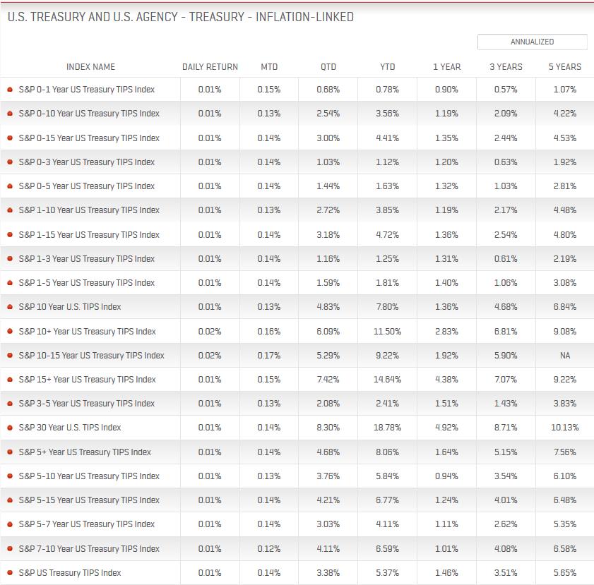
Source: S&P Dow Jones Indices, June 11, 2014
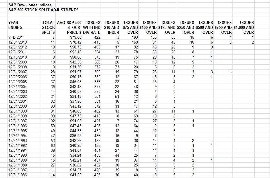Note: Though both indices measure 10 years they have not been duration matched.

Source: S&P Dow Jones Indices, June 11, 2014

This is a story about the power of randomness, and its application to investing.

A good few years ago, I had the pleasure of meeting Bob “The Rock” Cooper. Bob, an otherwise unassuming sales manager from London, had just won the world championship in the princely sport of “Rock Paper Scissors”. Yes, there is such a thing.

At the time I met Bob, I was working for the Royal Institution of Great Britain, which has hosted a series of “Christmas Lectures” presenting scientific concepts to a young audience every year since 1825, barring a brief interlude during the Second World War.

In 2006, the topic of the lectures was mathematics.¹  As one of the lectures was based on probability; we invited Bob in to talk about game theory, randomness and to try and beat him at Rock Paper Scissors.

Now, Bob’s pretty good at reading people’s intentions. He knows a good deal of behavioral psychology, and he plays a lot of Rock Paper Scissors. Unless you know as much as he does, whatever your strategy is, he’s going to beat you. He certainly could beat an 11-year old kid.

How do you beat Bob? You can’t determine a winning strategy, but you can improve your odds. If you play at random, you have a 50% chance of winning.  That’s as good a chance of beating him as he has of beating you – you’ve levelled the playing field.

What does this have to do with investing? Well, actually quite a lot. Think of the markets as Bob. They’re smarter than you, they’re good at exploiting your intentions, and if you try to beat them, on average you’re likely to fail. But if you play at random, you can improve your odds, potentially by a considerable margin.

Of course, I’m not recommending that investors should pick their investments at random. What we do recommend, however, is that investors keep an eye on the performance of equal weight indices. They tell you the performance of a random investment strategy. That’s convenient in terms of benchmarking: any “alpha” strategy worth its salt should outperform in comparison. Not many do.

1. If you’re interested, the full series is available here – although please be warned that the target audience is young children.

The key bar-room conversation this week has not been the stock market highs, or concern over elevated P/Es, or when a correction might arrive (the last one being in 2011 for big-caps), or even the increased M&A premiums being paid. It was stock splits, inspired by Apple’s 7-for-1 and the recollection, for those who have been on the Street for a few decades or more, and those newcomers who listened in, that in the 80s and prior, stock splits were money makers. Back then you actually paid cash for a service that sent a message (pre-twitter) to your beeper that a company had announced a planned split – and you would then purchase the stock – because it would go up (most likely).

The situation back then was that companies liked to keep their stock in a comfort zone, say $50 (for illustration), where investors felt comfortable buying and holding it. Additionally, old lots were inefficient in price and high in commissions (commissions were de-regulated in 1975, when brokerage consolidation slowly started and regulatory review was very show and long). Companies liked a broad base of individuals, which many felt gave support to the company; as compared to institutions which could be difficult (to put it nicely), or down-right unfriendly (Gulf & Devour). So when a stock reached a certain level, the company would split it, returning it to the comfort level (note: if $50 was the desired level, a 2-for-1 would most likely take place at $110 or higher, giving the company some protection in case the stock experienced a downdraft after the split – either because of company events or just market conditions). That thought process declined as quick trades came in along with the concept of capital appreciation only. Higher priced stocks were also becoming more acceptable, and the ability to purchase a dollar amount was made easier via brokerage consolidation, discount houses, and of course – the internet. Once we got past Y2K two recessions kept splits at bay (with the market sometimes splitting your stock in price, even though you did not get the extra shares).

Which brings us to Apple’s 7-for-1. There are many reasons why Apple split, but many believe it was to make its stock price, which was $646 per share before the split and $94 now, more attractive to individual investors, and broaden its investor base. Some even joked about a rebate program – buy a full-priced iPhone and get a share (not sure how that would work with disclosure or compliance). Also accepted was the idea that a border individual investor base could insulate the company from institutions and activists, who have been a bit more busy as company assets (especially cash) have grown. So, the question is – IF, yes IF, the lower price brings in more individuals (which would also add to buying and support the stock), and ‘assists’ with ‘dealing’ with certain holders, will more companies do it? Don’t know the answer, but as the Fed told the banks – I’ll be watching you.

And while we all know that June is the most popular wedding month, it also appears to be the most popular split month (don’t know about divorces – still happy with my first)

 Recent Splits: