Indexology^® Blog

The slope of the yield curve is a good recession predictor. When the curve is inverted – when the yield on three month T-bills is greater than the yield on the ten year T-Note – a recession is imminent. Similar signals can be seen if the T-bill is replaced by a two- or three-year T-Note or the Fed funds rate. The same result is found if one uses 20- or 30-year treasuries instead of the ten-year, although there is less data available for the longer maturities. The chart shows the spreads based on the ten-year note and either three-month bills or three-year notes. The vertical bars mark recession.

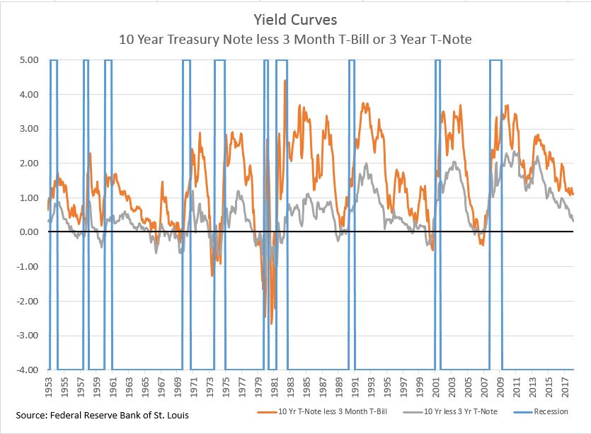
Currently the Fed is pushing the Fed funds rate upward and it is dragging other short term interest rates higher while the yield on the ten year note remains a touch below 3%. The yield curve isn’t inverted yet, but is headed that way.  Market expectations shown by trading in Fed funds futures point to two more increases in the Fed Funds rate this year, reaching a range of 2.25%-2.5% at year-end.  In his testimony today, Fed Chairman Powell said that gradual rate increases will continue.

Market commentary is focused on the yield curve trying to resolve the conflict between today’s strong economy and the yield curve’s warning.

For economic and monetary policy, the level of the real or inflation adjusted Fed funds rate matters as well as the relative positions of short and long interest rates. Normally the real Fed funds rate is positive. Over the last seven decades, it averaged 1.27%. When the real Fed funds rate is below zero, as it has been recently, monetary policy provides unusually large accommodation and support to the economy. That is why the Fed pushed the real funds rate into negative territory after the financial crisis. It is also a factor in the currently strong labor.  The second chart shows the yield curve based on the 10 year T-Note and 3 month T-bill and the real Fed funds rate.

Before almost every recession, as the yield curve inverted the real Fed funds rate climbed sharply higher. The exception was the short recession in 1980 followed by a failed recovery and a second recession within 12 months. As long as the real funds rate remains in negative territory, analysts can temper their anxiety over the yield curve.  Today the real Fed funds rate is -1.0% while the Fed’s current range for the nominal rate is 1.75%-2%. The recent Monetary Policy Report from the Fed suggests that the nominal Fed funds rate range will top 3% in 2019, pushing the real rate into positive territory as long as the inflation goal holds. There will always be another recession. The next one may not be as soon as the yield curve hints.

This week I am participating in a retirement panel at the University of Chicago Booth School of Business with key thought leaders from the Plan Sponsor Council of America, the Employee Benefits Research Institute and S&P Dow Jones Indices.  The panel, moderated by my good friend Jody Strakosch, creator of one of the first DC retirement income products, will focus on applying goals-based investing to default investments in DC plans.

In this blog, I discuss my thoughts on the impact of one’s human capital—the present value of lifetime earnings—on retirement plan design. Bob Merton, Bill Samuelson, and I were the first theorists to rigorously model this factor in our 1992 paper entitled Labor Supply Flexibility and Portfolio Choice in a Life-Cycle Model, (Journal of Economic Dynamics and Control, 1992). That paper influenced all subsequent theoretical and practical discussions on the topic.

The key insights were the following:  First, the ultimate objective is to save enough during one’s working years to maintain a standard of living in old age after human capital is exhausted.  Second, the optimal fraction of one’s retirement portfolio allocated to equities depends on the amount of remaining human capital (age) and equity exposure through one’s job.  For example, the human capital for a tenured professor is less risky than that of a worker in a cyclical industry.  The ability to adjust one’s age of retirement is a key factor in the optimal allocation to equities during the working years. In general, the greater the market-risk exposure of one’s job, the lower the fraction to invest in equities.

Since default investments tend to be designed for all workers during all phases of retirement planning we must seek to accumulate enough retirement assets and manage market risk exposure to achieve a target level of income in retirement.  When we are young, say right out of college, most of us have a small amount of financial capital (potentially negative if we still have education debt), however over time we gain financial capital by saving as we enter our peak earning years.  Therefore, based on this assumption, lifecycle asset allocation should evolve over time, potentially from a high allocation to equities to a portfolio that produces a reliable stream of inflation-proof income.

For more on this subject, I recommend other blogs addressing retirement income, such as the recent post by my fellow panelist, Jodie Gunzberg of S&P Dow Jones Indices: https://www.indexologyblog.com/2018/04/19/standard-benchmarks-extend-standard-of-living-through-retirement/.  If we adopt the mantra that income is the outcome, goals-based investing is the investment approach that helps our industry design the right default solutions for all workers, at all times.

Q2 2018 showed that volatility is king in Latin America. The first quarter saw strong returns for the region, with Mexico lagging. In the second quarter, we saw a practical wipeout of all gains for the year and a return to negative territory for Latin America. Recent presidential elections in Mexico and Colombia, as well as upcoming elections in Brazil brought economic uncertainty. Brazil, the largest market in the region, had a significantly tough second quarter. During this period, the country saw great currency depreciation, climbing inflation rates, as well as fiscal and political challenges that largely contributed to the region’s plunge. For the quarter, the S&P Brazil BMI was down 26% in U.S. dollar terms, while the regional S&P Latin America BMI and S&P Latin America 40 were down 18% and 19%, respectively.

It is indisputable that Latin America is going through major upheavals. However, in terms of indices, one of the factors with the biggest impact is currency fluctuations. All the local and regional indices saw sharp drops in performance when looking at U.S. dollar returns, while local investors saw a different picture of the region. A good example is the S&P MILA Pacific Alliance Composite, which excludes Brazil. The broad region of 141 stocks saw returns of -5% in USD for the quarter, but in Chilean and Mexican pesos, the returns were positive, up 2.7% and 2.5%, respectively. In Colombian pesos, the index was flat at 0.1% and in Peruvian nuevos soles, it was down 3%. This shows that, depending on where you are, currency plays an important part in index performance.

Despite the underperformance, there were some strong positive returns, particularly in Mexico and Colombia. The S&P/BMV IPC and S&P Colombia Select displayed strong performance in local currency terms, generating returns of 4.4% and 10.4%, respectively. Other pockets of positive returns were in the energy sector of the Pacific Alliance region,[1] which returned nearly 4% for the quarter and 64% for the year ending June 2018 in U.S. dollar terms.

Volatility is the name of the game in Latin America, and it will be interesting to see what happens next quarter. So far, the presidential elections in Mexico have barely had any impact on the market, and in the first week of July, Brazil has come back to positive territory, but there are many weeks still ahead before the next quarter—stay tuned.

To see more details about performance in Latin America, please see: S&P Latin America Equity Indices Quantitative Analysis Q2 2018.

[1] The Pacific Alliance region includes Chile, Colombia, Mexico, and Peru.

In January 2003, S&P Dow Jones Indices introduced the world’s first equal-weighted index, the S&P 500^® Equal Weight Index, leading the way for the subsequent development of non-market-cap weighted indices.[1] Since then, looking at the index’s historical back-tested performance, it outperformed its market-cap-weighted counterpart, the S&P 500, in 16 out of 28 years, with an annualized excess return of 1.44% per year.[2]

In addition to better relative performance, equal weighting can have fundamental appeal for market participants who subscribe to the notion that market-cap weighting exhibits momentum bias, with winners getting a larger weight in the index, and potentially leading to concentration and overvaluation issues. Therefore, for those who wish to reduce concentration risk or to separate the price of a security from its fundamentals, an equal-weight index can offer an alternative approach.

Moreover, equal-weight indexing could hit closer to home for proponents of passive indexing, given that its investment underpinning runs counter to active investing. While active management seeks to exploit risk and return expectations of securities through a superior selection process and diversified portfolio construction, equal-weight indexing assumes that all the securities in the universe have the same expected returns and volatility. In other words, by equal weighting, we assume that an average investor has no forecasting ability or is unable to distinguish securities’ returns and volatilities.

Therefore, one can argue that the lack of return, risk, and covariance matrix assumptions in an equal-weighted index makes it a natural benchmark against actively managed funds that incorporate all those expectations. In fact, several studies have shown that an alpha-generating strategy should be able to outperform an equal-weight benchmark.[3]

Against that backdrop, we compare the performance of actively managed U.S. large-cap and large-cap core funds with the S&P 500 Equal Weight Index (see Exhibits 1 and 2) as of March 31, 2018.[4] As we can see below, over the near-term horizons (one, three, and five years), a higher percentage of large-cap funds underperformed the S&P 500 than the S&P 500 Equal Weight Index, primarily due to mega-cap securities performing well in the large-cap space and contributing significantly to the S&P 500 returns over the past two years.

However, over the long-term investment horizons (10 or 15 years), a greater percentage of large-cap funds underperformed the S&P 500 Equal Weight Index than the S&P 500. In fact, the 15-year figures paint a difficult landscape in which close to 100% of large-cap managers underperformed the S&P 500 Equal Weight Index.

Our analysis shows that the S&P 500 Equal Weight Index set a higher threshold for managers to outperform in the long run. In a subsequent blog, we will look at the underlying risk factor exposures of the S&P 500 Equal Weight Index and present a framework in which the index can serve as a supplementary benchmark to evaluate large-cap managers.

[1]   Zeng, L. and Luo, F. “10 Years Later: Where in the World is Equal Weight Indexing Now?” S&P Dow Jones Indices LLC. April 2013.

[2]   Calendar year returns were calculated from 1990 through 2017. Annualized excess returns were computed from Jan. 31, 1990, to May 31, 2018. Past performance is no guarantee of future results. Hypothetical performance is used.

[3]   Edwards, T. and Lazzara, C. “Equal-Weight Benchmarking: Raising the Monkey Bars.” S&P Dow Jones Indices LLC. May 2014.

[4]   For our analysis, the underlying data source was the University of Chicago’s Center for Research in Security Prices (CRSP) Survivorship-Bias-Free US Mutual Fund Database, which is the same source used by the headline SPIVA^® U.S. Scorecard.