Indexology^® Blog

For corporate bond managers, credit analysis is a key step in the investment process, one that lays the foundation for their credit outlook and investment strategies. Credit analysis assesses bond issuers’ creditworthiness and evaluates their ability to make timely interest and principal payments. Credit analysis is critical in helping bond managers assess the state of the credit cycle we are in, select bonds of healthy credit quality, and avoid names that could potentially suffer large principal loss. The analysis includes qualitative and quantitative components. On the quantitative side, credit ratios that measure leverage, interest coverage, liquidity, and profitability allow for the evaluation of a bond issuer’s financial risk profile.

Can we incorporate credit analysis into a rules-based methodology to capture some of the alpha and/or mitigate credit risk generated by active portfolio management? Credit ratio analysis, being quantitative, offers such an opportunity. To do so, we propose a rules-based model that uses credit ratios to screen out the least creditworthy issuers, thereby constructing a corporate bond portfolio with strong credit quality. We acknowledge that ratio analysis is only one part of credit analysis, and though necessary, it is not sufficient to assess an issuer’s creditworthiness. Therefore, instead of actively selecting companies with healthy ratios, we seek to use credit ratios to screen out companies at the bottom of the ranks, indicating financial stress.

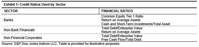
The methodology involves two steps. First, we construct a representative investable universe from the broad investment-grade and high-yield corporate bond universe, respectively, by applying criteria on bond size (minimum size of USD 750 million for investment grade and USD 400 million for high yield), maturity (2 years-10.5 years), and spread duration (greater than or equal to 1). In line with the objective of constructing a quality credit portfolio for the high-yield universe, we exclude bonds with a credit rating below “B-.” Second, we group bond issuers by sector (banks, non-bank financials, and non-financial corporates), and use a set of sector-specific credit ratios on leverage, interest coverage, liquidity, and profitability to rank issuers within sectors (see Exhibit 1).

For the applicable ratio within each sector, we calculate a trimmed z-score for every issuer and then standardize the scores within the sector. We rank issuers by the average of the standardized z-scores within their respective sector. The bottom 20% of issuers in each sector are then screened out. The remaining issuers are equally weighted, and bonds issued by the same issuer are equally weighted in the portfolio. The portfolio rebalances quarterly at the end of February, May, August, and November each year.

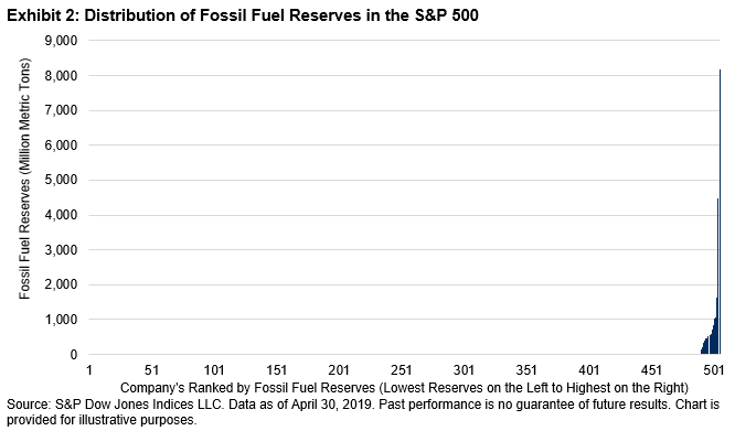
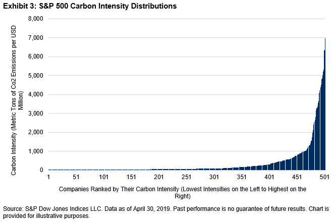
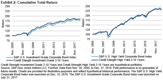
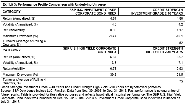
Exhibits 2 and 3 compare the back-tested performance of the credit strength portfolios with the underlying broad market indices. For investment-grade and high-yield bonds, credit strength portfolios reduced return volatility and improved risk-adjusted returns. The maximum drawdown was lower than the underlying universes during market downturns.

The back test shows that incorporating credit ratio analysis in a rules-based portfolio construction process resulted in potentially more desirable risk/return characteristics for investment-grade and high-yield corporate bonds. In our next blog, we will further explore the benefits of downside protection and sector diversification that the credit strength strategy offers.

The performance of U.S. equity factors during Q2 was lackluster, with most underperforming the S&P 500, as seen in Exhibit 1.  While Minimum Volatility and Low Volatility were notable exceptions, Value, Quality, High Beta, and Momentum all lagged the benchmark – in large part because of their tilt toward smaller companies.  Since most factor indices are not cap-weighted, their out- or under-performance tends to parallel that of the equal-weighted 500.

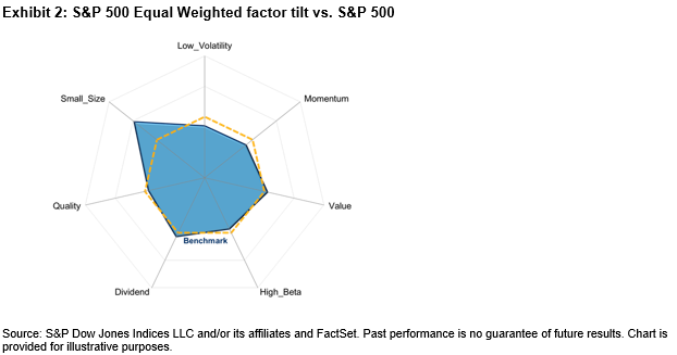
  Equal Weight is a particularly good illustration of the small-size effect, since it holds the same stocks as the cap-weighted S&P 500.  Exhibit 2’s factor exposure chart makes Equal Weight’s small cap tilt clear.  Given the outperformance of larger-cap stocks during the quarter, Equal Weight performance was understandably disadvantaged.

Exhibit 3 demonstrates that larger-cap stocks dominated within most sectors of the S&P 500, with a particularly noticeable effect in the Consumer Discretionary and Info Tech sectors.  Seven out of eleven equal weight sectors underperformed their cap-weighted counterparts.

The S&P 500 Pure Value Index provides a less direct example of the impact of large-cap performance. The key driver of Pure Value’s underperformance last quarter was stock selection, again primarily in the Info Tech and Consumer Discretionary sectors.

Active managers are not immune to these effects.  Our SPIVA database shows that active management tends to be particularly challenged in periods when the largest stocks outperform, and when Low Volatility outperforms.  If I were a betting woman, I would not bet on active manager outperformance when our next SPIVA report appears.

“Sustainable investing must go mainstream. Fortunately, the momentum is growing.” – Mark Carney

Mark Carney’s statement underpins the sentiment of the investment community, where environmental, social, and governance (ESG) considerations have entered the forefront of investors’ priorities.

Whether factor indices have ESG principles integrated or not, understanding a factor’s influence on ESG characteristics, such as the benefits of quality, can be advantageous.

Exhibit 1 presents a heat map visualizing the S&P Factor Indices’ ESG exposures. This can be interpreted as red representing poor performance, yellow as middle, and green as strong, relative to the other indices.

Using S&P DJI ESG Scores, ESG improvements from the parent index were calculated as a percentage of possible ESG improvement if the total index weight were to be placed in the highest ESG-scoring stock (hence, there is no data for the S&P 500^® as it is the benchmark for the factor indices analyzed). The S&P DJI ESG Scores are based on underlying data from SAM’s award-winning Corporate Sustainability Assessment combined with an S&P DJI methodology of how underlying data is treated and aggregated.[1]

The “ESG,” “E,” “S,” and “G” columns in Exhibit 1 refer to the improvement in the ESG, environmental, social, and governance levels of the S&P DJI ESG Scores, while the other columns refer to various Trucost carbon footprinting methods.

Exhibit 1 illustrates that factor exposures can have a strong influence on ESG scores.

Quality topped all factors, showing strong ESG performance, fossil fuel reserves aside. Fossil fuel reserves, however, are driven largely by one company, Occidental Petroleum—only four companies included in the S&P 500 have any fossil fuel reserves. The nature of this metric, with only 16 S&P 500 constituents having fossil fuel reserves recorded by Trucost (see Exhibit 2), means the figure is skewed by including just one high fossil fuel reserve company. On the S&P DJI ESG Score front, quality performs well, seeing an ESG performance increase almost as high as the S&P 500 ESG Index, albeit with a stock count of less than a third.

Alternately, the S&P 500 Low Volatility Index shows the poorest ESG characteristics, with a 29% ESG reduction, largely driven by a 41% environmental reduction, while also falling short on social and governance factors. These S&P DJI ESG Scores[2] are backed by poor carbon to value, carbon to revenue, and weighted average carbon intensity figures, which were the worst performers of the factor indices analyzed. The low carbon scores are unsurprising, considering the large number of Utilities companies with low volatility characteristics. Exhibit 3 illustrates the distribution of carbon intensities, heavily skewed as with the fossil fuel reserves.

A responsible investor may consider implementing a carbon reduction strategy for a low volatility index or combining ESG with low volatility to gain stronger ESG exposures while still capturing the low volatility risk premia. In the next blog, we’ll see what drives these scores, as well as how constant the sector allocations within factor indices are over time.

[1]  “S&P DJI ESG Scores FAQ,” S&P Dow Jones Indices.

[2]  “Index ESG Characteristics Explained,” S&P Dow Jones Indices.

The second quarter of 2019 reinforced the upside potential of S&P MARC 5% Excess Return (ER) Index diversification, which compliments traditional risk management benefits. With the equities and fixed income components having good, but not stellar, Q2 performance, we have to look to gold to understand the driver of the S&P MARC 5% (ER) Index’s performance. Gold, as measured by the S&P GSCI Gold, started the quarter primarily in negative territory but turned positive toward the beginning of June and rose significantly on the back of a dovish Fed.

With all three component indices within the S&P MARC 5% (ER) Index ending positive on the quarter, much of the gain in gold occurred between June 19, 2019 and June 20, 2019, when the Fed released its newest policy statement and, just as importantly, its interest rate projections. The lift in gold contributed significantly to the performance of the S&P MARC 5% (ER) Index for Q2 2019, with the weighted return for the single day contributing 1% to the S&P MARC 5% (ER) Index.

When looking at the relative returns of the components of the S&P MARC 5% (ER) Index versus the index itself, you can observe that the diversification still held in Q2 2019, though the index also managed to capture relatively sizeable shifts in any given asset class. This can best be seen toward the right side of the chart, where the outsized relative performance caused equities and fixed income to underperform the S&P MARC 5% (ER) Index, despite each being positive for the quarter (see Exhibit 3).

Looking at the rolling 252-day performance for the 63 days in the quarter, we can see that for any of the 252-day periods, the return of the S&P MARC 5% (ER) Index would have been positive despite the inconsistencies in most of its components. It is also worth noting that, because of the diversification of the index, during the past few observation periods ending in June 2019, the S&P MARC 5% (ER) Index also outperformed each of the individual asset classes over the 252-day period.

Commodities markets resumed their upward trajectory in June. The S&P GSCI was up 4.4% for the month and up 13.3% YTD. The Dow Jones Commodity Index (DJCI) was up 3.1% in June and up 6.9% YTD, reflecting its lower energy weighting. A recovery in petroleum prices and an impressive rally in gold were the main drivers of the broad commodities indices’ performance over the month.

In the oil markets, bearishness regarding the state of the global economy was tempered by fears regarding a possible disruption of oil exports from the Gulf region and prospects for a renewed production deal from OPEC. Tanker attacks in the Strait of Hormuz and the Gulf of Oman over the course of June undermined global shipping security and escalated the dispute between the U.S. and Iran over its nuclear program. The S&P GSCI Petroleum ended the month up 7.2%. At the start of July, a deal was reached between members of the OPEC Plus group to extend the existing oil output cuts of 1.2 million barrels per day for nine months.

The S&P GSCI Industrial Metals reversed its course from the prior two months, rising 2.0% in June. Over the first six months of the year, the S&P GSCI Nickel rose an impressive 19.1%; the rally was largely attributed to the long-term prospects for the use of nickel in electric vehicles and falling exchange-held inventories, and was in spite of the fact that the well-documented supply gap in the refined nickel market is expected to shrink over the second half of the year. The S&P GSCI Iron Ore moved significantly higher, by 14.9% in June, due to another drop in port inventories and additional Chinese government stimulus. An agreement between Trump and Xi Jinping to restart trade talks following a meeting at the G20 Summit also contributed to the strong performance.

The other metal to record double digit percentage gains was the S&P GSCI Palladium, which jumped 15.7% in June due largely to investor demand and is now close to reaching an all-time high. The S&P GSCI Gold increased 8.0% for the month. The exhilaration that was associated with the strength of the global economy a year ago has been replaced with growing financial market turbulence, a plethora of geopolitical flashpoints, and a string of economic releases that have fallen short of expectations. It would appear that few central banks wish to find themselves on the wrong side of the U.S. Fed, suggesting that lower interest rates are on the horizon. Gold tends to perform well in these circumstances.

The S&P GSCI Agriculture ended the month up only 0.3%, with some of the recent weather-induced exuberance taken out of the grains market on the last day of the month, following the release of the USDA’s Acreage Report. The S&P GSCI Coffee was up 2.2% in June, with prices buoyed by the threat of a cold snap in Brazil, which could pose a threat to crops.

The rollercoaster ride continued in the lean hogs market, with the S&P GSCI Lean Hogs down 10.0% in June. The latest U.S. hogs and pigs report indicates that pig and pork supplies in 2019 will be well above last year’s levels. The June 2019 hog inventory was up 4% year-over-year and the breeding herd expanded by 1%. This is the highest June 1 inventory of all hogs and pigs in the U.S. since estimates began over 50 years ago. At the same time, U.S. pork exports to China have been lackluster due to the ongoing trade spat between the two nations, and despite the devastation caused to the Chinese domestic industry by African swine flu.