Indexology^® Blog

Dividends and stock buybacks are two ways that a company returns capital to its shareholders. Investors can benefit from both, but is there a synergy that can result from combining them?

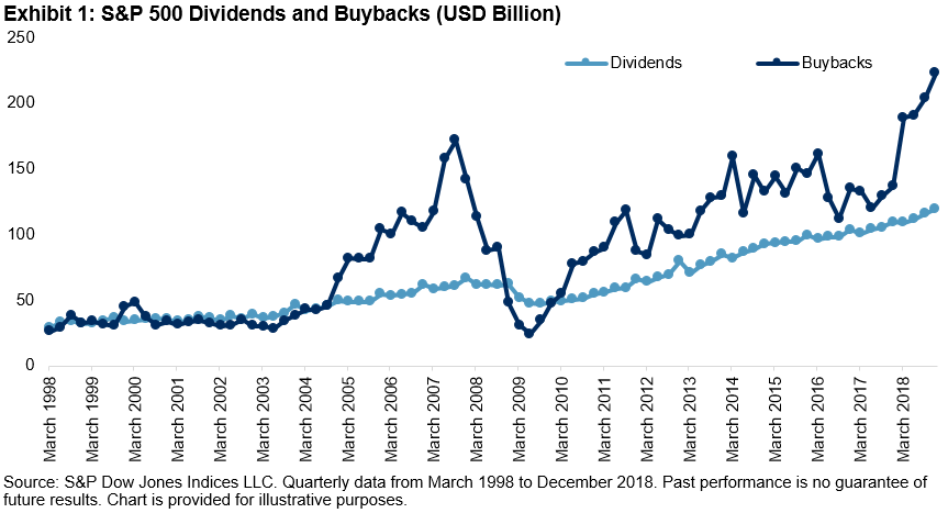
We’ve seen a surge in both buyback value and the number of participating companies in recent years. In 2018, 444 of S&P 500^® companies spent USD 806 billion on buybacks.[1] Additionally, more dividend-growing companies have begun repurchasing shares while consistently increasing dividend distribution. Exhibit 1 shows this trend in the S&P 500 Dividend Aristocrats^®.

To evaluate the two forms of shareholder payouts, we compared dividend yield[2] and buybackyield[3] (see Exhibit 2). Buyback yield was significantly lower than dividend yield before 2003 and became quite unstable until the end of the financial crisis. From then on, buyback yield surpassed dividend yield.

Choosing between dividends and share repurchases is a contentious debate. Income-oriented investors may prefer dividends, while growth-oriented investors may desire the capital appreciation that buybacks bring. Although either payout strategy can benefit investors over time, an alternative and holistic strategy would be to integrate the two.

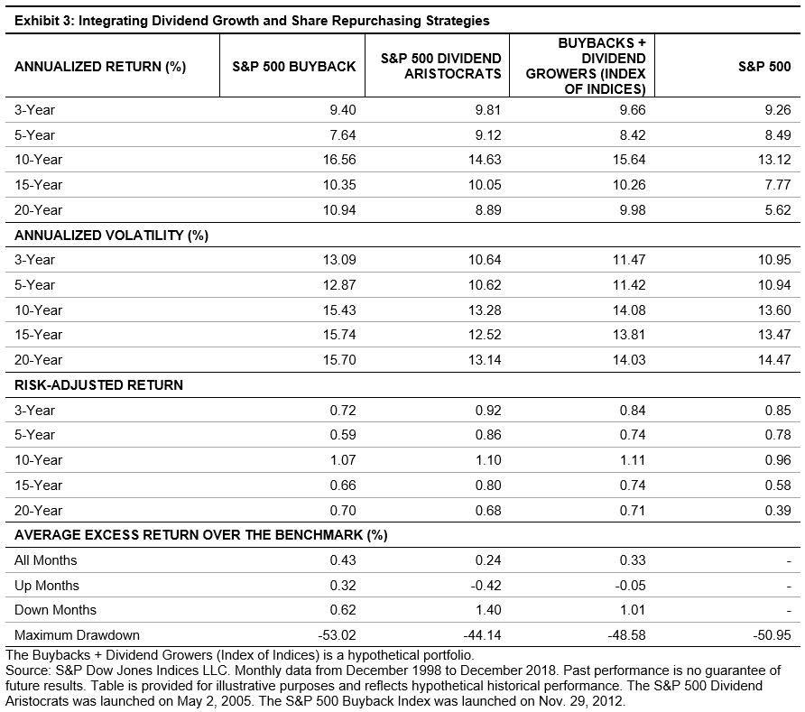
Using the S&P 500 Buyback Index[4] and the S&P 500 Dividend Aristocrats,[5] we formed a hypothetical portfolio of companies with sustainable dividend yield and high buyback yield. The hypothetical index of indices approach is a simple guideline because there is a possibility of overlap between the two strategies. However, we find that overlap between the two indices is fairly low—6.4% on average when measuring on a quarterly basis from December 1998 to December 2018. The combined strategy does indeed display the highest risk-adjusted return over the long-term investment horizon (see Exhibit 3), indicating that investors could benefit from integrating both factors.

[1] “S&P 500 Q4 2018 Buybacks Set 4th Consecutive Quarterly Record at $223 Billion,” S&P Dow Jones Indices.

[2] Dividend yield is the annual dividend amount relative to the market value.

[3] Buyback yield is the stock buyback value relative to the market value.

[4]   The S&P 500 Buyback Index is designed to measure the performance of the top 100 stocks with the highest buyback ratios in the S&P 500. For more information, please visit https://spindices.com/indices/strategy/sp-500-buyback-index.

[5]   The S&P 500 Dividend Aristocrats is designed to measure the performance of S&P 500 companies that have increased dividends every year for the last 25 consecutive years. As of March 29, 2019, the index contains 57 issues. For more information, please visit https://spindices.com/indices/strategy/sp-500-dividend-aristocrats.

In general, it is a positive sign when a company buy back shares. This means the company believes its stock is undervalued and is confident about its future earnings. In recent years, buybacks have become increasingly popular. With a record number of companies buying back shares, how are these companies are faring?

A company can choose to return value to shareholders in a number of ways: it can pay out cash dividends, reinvest in the business, buyback shares, or a combination of these.[1] Traditionally, paying out dividends has been the dominant method to return a company’s excess cash to investors, and dividend income returns have contributed to over one-third of the monthly total return of the S&P 500 from 1928 to 2016.[2] In a share repurchase, a company reduces its shares outstanding through an open-market buyback or tender offer.

Exhibit 1 charts the aggregate amount of dividends and repurchases of S&P 500 companies since 1998. While cash dividends show a steady increase over time, the amount of shares repurchased has been volatile. The amount of buybacks jumped significantly right before the 2008 global financial crisis and dropped drastically in 2009. Since 2010, the amount of buybacks has continuously grown and exceeded the amount of dividend distributions.

The buyback momentum has continued into 2019, even after a record USD 806 billion[3] buyback in 2018, a 56% increase from the previous year. As shown in Exhibit 2, two decades ago, fewer than half of S&P 500 companies purchased shares back. The participation rate stood at around 80% as of Dec. 31, 2018.

Since its inception in January 1994, the S&P 500 Buyback Index returned 13.29% annually, compared with gains of 10.31% and 8.96% from the S&P 500 High Dividend Index and S&P 500, respectively. One of the key reasons for the outperformance is that buying shares back decreases the company’s shares outstanding, which helps improve earnings-per-share (EPS) and eventually propels stock prices higher.

[1]   Zeng, “Examining Share Repurchasing and the S&P Buyback Indices in the U.S. Market” (April 2016)

[2]   Li and Soe, “Incorporating Free Cash Flow Yield in Dividend Analysis” (November 2017)

[3]   “S&P 500 Q4 2018 Buybacks Set 4th Consecutive Quarterly Record at $223 Billion,” S&P Dow Jones Indices

LIBOR – the London Interbank Offered Rate — is the benchmark for over $300 trillion of loans, derivatives and other financial instruments.  LIBOR started in the syndicated loan market of the 1960s; today it is quoted in different currencies and maturities. Following scandals in 2012-2013, LIBOR is being replaced and will disappear in 2021.

For US dollar denominated loans and derivatives, the replacement for overnight LIBOR will be SOFR (Secured Overnight Financing Rate). It is based on overnight REPOs used by the Fed as part of its interest rate management. The New York Federal Reserve bank began publishing SOFR this time last year. Other overnight rates are being established covering the UK, Europe, Switzerland and Japan. (See the table.)  Initially these will be quoted as overnight rates only; regulators and industry groups are beginning to discuss term rates for maturities longer than overnight.

Originally, London-based banks set LIBOR by sharing estimates of what each bank could expect to pay for to borrow overnight money without collateral. Today’s process is more formal, however LIBOR continues to be partially based on estimates of what overnight funding would cost a recognized bank. SOFR has two key differences: it is calculated from actual trades, not estimates. It is a secured rate based on REPOs of US treasury securities.  Over time, SOFR may drop below LIBOR since it is a secured rate. Further, in a crisis a secured rate like SOFR rate could fall while an uncollateralized rate like LIBOR rises.

In 1986, when LIBOR was well established and widely used, the British Bankers Association, with the support of the Bank of England, formalized the LIBOR rate setting and changed the process to exclude the highest and lowest quotes in each setting. Beginning in 2007 there were rumors and articles in the press raising questions about the LIBOR process and suggestions that a bank might quote low rates to enhance its credit quality. In 2012, several banks were found to be manipulating the rate to their own advantage. A year later in 2013 the European Union levied financial penalties totaling over $2 billion against a group of eight major banks. SOFR and other LIBOR replacements use of actual trades from liquid markets to prevent a repeat of the scandals that plagued, and then, brought down LIBOR.

The chart shows the Fed funds rate, US dollar overnight LIBOR and SOFR over the last year. SOFR tends to move sharply at quarter-ends when banks look to the repo market for window dressing. As more funds focus on SOFR, it may become less volatile.

The methodology of the S&P BSE SENSEX has seen many changes over the last 30 years. In October 2018, it was again modified after an extensive market consultation.

The recent changes brought new clarity to the boundaries for entry and exit of stocks in the index. Constituents are selected by size and liquidity. Now, any constituent with a free-float market cap rank beyond 39 will be dropped from the index and any non-constituent with a rank equal to or less than 21 will qualify for inclusion in the index. This helps the S&P BSE SENSEX methodology become rules-based, transparent, and objective.[1]

Using the new methodology as a part of the semiannual index reconstitution, Asia Index Private Ltd (a joint venture between S&P Dow Jones Indices and BSE Ltd) announced changes to the S&P BSE SENSEX composition on November 22, 2018. Bajaj Finance (a leading non-banking finance company company) and HCL Technologies (a leading global information technology company) replaced Wipro and Adani Ports and Special Economic Zone (see Exhibit 1). These changes were effective as of the market open on December 24, 2018.

The S&P BSE SENSEX noted total returns of 7% over the three months since the previous rebalance. During this period, new members Bajaj Finance and HCL Technologies outperformed the index by 2.5% and 0.6%, respectively, on a total returns basis. Good though this outperformance is, it had a minor effect of 0.27%, combined, on the index’s total return, on account of the two new companies’ small weight in the index.

Source: Bloomberg and Asia Index Private Limited. Contribution and total returns from Dec. 21, 2018, to March 22, 2019. Weight as of rebalance as of Dec 21, 2018. Past performance is no guarantee of future results. Table is provided for illustrative purposes.

Historically, India’s equity market has been dominated by the Financials sector, and this is also true of the S&P BSE SENSEX. The weight of Financials in the index before the October 2018 changes was 41.5%. It increased by 1.3% to 42.8% on account of the inclusion of Bajaj Finance. The Industrials sector noted a fall of 0.9% in sector weight with the exclusion of Adani Ports and Special Economic Zone.

Source: Asia Index Private Limited. Weights as of Dec. 21, 2018. Table is provided for illustrative purposes.

The S&P BSE SENSEX, India’s most tracked bellwether index, is designed to measure the performance of the 30 largest, most liquid, and financially sound large-cap companies across key economic sectors of the Indian economy. The index represents approximately 44% of BSE-listed companies in terms of total market capitalization. It follows a free-float-adjusted, market-cap-weighted methodology and is reviewed semiannually in June and December.

[1] For detailed methodology please visit www.asiaindex.co.in.

The SPIVA^® U.S. Year-End 2018 Scorecard shows a reversal of the relative short-term performance of fixed income funds at the end of 2018 from six months prior. Combined with the interest rates move, this might shed some light on understanding the duration positioning of active funds.

We focus on government bond funds for our analysis, since duration positioning is the most important directional exposure for this type of strategy. Exhibits 1 and 2 show changes in interest rates alongside the relative performance of government bond funds as compared to their benchmarks, using one-year gross returns.

When the bond markets changed direction from a sell-off in the first half of 2018 to a rally in the second half, the percentage of short and intermediate bond funds underperforming their benchmarks increased significantly, from 22% and 11%, to 52% and 65%, respectively. At the same time, the reverse happened to long-end government bond funds. These quick inversions of performance may indicate that most short and intermediate bond funds were underweighting duration going into the second half, and the ensuing bond rally caught active bond managers by surprise.

Yet the SPIVA Year-End 2018 showed consistent underperformance from more than half of the funds in most of the taxable bond fund categories over the mid- and long-term periods. For example, as of the end of 2018, more than 50% of such funds underperformed their benchmarks on five-year net return.  This divergence between short- and long-term relative performance by taxable bond managers is not unique in the history of SPIVA.

Exhibit 3 shows the percentage of fixed income funds underperforming benchmarks historically on one-year and five-year bases, where the red text indicates years when more than 50% of the funds lagged benchmarks. More than 50% of the funds outperformed their benchmarks occasionally over the one-year basis, but it was less common over the five-year horizon.

The latest SPIVA U.S. report shows that more than 50% of short and intermediate bond funds underperformed their benchmarks after outperforming six months ago. Our analysis shows that on a five-year return basis, such a switch of relative performance was unusual, as underperformance was persistent.