Indexology^® Blog

In a previous blog, we took the first and second steps in our Growth at a Reasonable Price (GARP) strategy construction. We introduced the GARP investment strategy and showed how it can be implemented systematically. In this blog, we will take the third and fourth steps: using a multi-factor sequential filtering process for security selection and establishing constituent weights.

Multi-Factor Sequential Filtering Process

There are a number of approaches one can take to construct multi-factor portfolios—mainly integration,[1] sequential filtering, and optimization. We use the sequential filtering method because it is easy to understand and effective in achieving its targeted factor exposures.

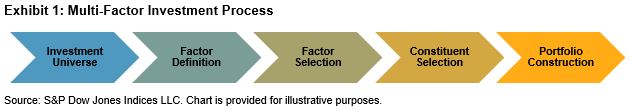
Multi-factor sequential filtering selects stocks using two layers of filters, as shown in Exhibit 1. In the first step (filter 1), stocks are ranked by their growth z-scores, with the top 150 stocks remaining eligible for constituent inclusion. In the second step (filter 2), those 150 stocks are then ranked by their quality & value (QV) composite z-scores. The top 75 stocks are selected to be included in the strategy after applying a 20% buffer rule.[2] The 20% buffer is applied to reduce portfolio turnover.

Constituent Weights

Once constituents are selected at each rebalance, eligible securities are weighted by their growth score[3] to achieve the strategy’s growth exposure. To limit the impact of extreme values, the maximum weight of a security is capped at 5%. Individual GICS^® sector exposure is capped at 40% to broaden the strategy’s sector exposure.

In this and a previous blog, we discussed our GARP strategy construction process. In coming blogs, we will present the empirical results of the strategy performance, its sector composition, and its performance attribution.

^[1]   S&P Quality, Value & Momentum Multi-Factor Indices Methodology, February 2019.

[2]   Buffer Rule: A 20% buffer is implemented as follows:

1. Stocks in the top 150, based on growth z-score, are ranked by their QV composite z-score. The top 60 stocks are automatically chosen for index inclusion.
2. Stocks that are current constituents that fall within the top 90 based on their QV composite z-score are chosen for index inclusion in order of their QV composite z-score.
3. If at this point 75 stocks have not been selected, the remaining stocks are chosen based on their QV composite z-score until the target count is reached.

[3]   Please see Footnote 7 from the last blog for growth score computation.

At the recent Australian Indexing & ETF Masterclass series held in Melbourne & Sydney, we asked the audience, 83% of whom were Financial Advisers, a number of questions using a mobile-enabled polling tool. Over 260 people attended the Masterclass across the two cities, and 189 of these people used the polling tool. 767 discrete votes were received across the six polls that we conducted. The results provide a snapshot of Financial Adviser views on ETFs, current usage, planned future usage and the prime considerations in selecting ETFs. Let’s look at the results in detail.

Our first poll asked the audience to nominate a range that represented their usage of ETFs in client portfolios. The largest response was for the highest range.

1. A full 29% of advisers indicated that between 76-100% of their client portfolios use ETFs;
2. 12% of respondents indicated that their client portfolios use between 51-75% ETFs; and
3. 24% of respondents polled said that between 26-50% of their client portfolios were ETF driven.

These results combined indicate that 65% of advisers are using ETFs for at least 25% of their client portfolios.

Our second poll question asked attendees the split between Australian-listed vs internationally-listed ETFs used in client portfolios. The splits reported were as follows:

1. 16% of respondents only use Australian-listed ETFs;
2. 16% of respondents mainly use Australian-listed ETFs;
3. 46% of respondents split usage 50:50 between Australian-listed and internationally-listed ETFs;
4. 18% of respondents mainly use internationally-listed ETFs;
5. 4% of respondents only use internationally-listed ETFs.

Our third poll sought to ascertain the indexing and ETF topics in which attendees are most interested. The results came out as follows:

1. 35% of poll responses nominated Equities & Sectors;
2. 22% nominated Smart Beta/Factors;
3. 15% nominated Fixed Income;
4. 13% went for ESG; and
5. 10% put their hands up for Commodities.

We also asked attendees, whether they expect their usage of ETFs to increase over the next 12 months:

1. 76% indicated their use of ETFs will increase;
2. 21% indicated there would be no change in use; and
3. 3% indicated their use of ETFs will decrease.

When asked a follow up question, as to the expected increase in ETF use over the next 12 months respondents provided the following results:

1. 12% expect to increase usage by 81-100%;
2. 12% expect to increase usage by 61-80%;
3. 20% expect to increase usage by 41-60%;
4. 32% expect to increase usage by 21-40%;
5. 22% expect to increase usage by 1-20%; and
6. 2% expect no increase in their use of ETFs.

Our final poll questions to the Masterclass audience asked what their prime considerations are when selecting ETFs. The results were as follows:

1. 32% look to the ETF issuer’s reputation in making a selection;
2. 22% look at the liquidity of the ETF and 22% also consider the expense ratio;
3. 13% consider past performance; and
4. 10% consider the Index provider’s reputation.

These results, pleasingly, demonstrate that there is a propensity to increase the use of ETFs as tools within client portfolios to achieve investment objectives. While just over 1/3 of respondents nominated Equities and Sectors as their topic of greatest interest, it is also pleasing that other topics have a solid level of interest also, indicating, that while equities are the core of ETF use, other asset classes are also on advisers’ radar.

The responses also provide valuable insights into the topics that we can address at future adviser-facing events, including our 10^th Annual Indexing and ETF Masterclass scheduled for Q1, 2020.

In case you missed our country classification announcement on Dec. 5, 2018, we will be starting the process of adding China A-shares to S&P DJI global benchmarks (including the S&P China BMI and S&P Emerging BMI) in September 2019 at a partial inclusion factor of 25%.

Given the size of China’s onshore equity market, the addition of China A-shares is a landmark event for the S&P Global BMI. Based on total market capitalization—unadjusted for foreign ownership limits and float adjustment—China is the world’s second-largest stock market and is nearly double the size of Japan and three times the size of the UK.

What exactly is happening? Effective at the market open on Sept. 23, 2019, China A-shares accessible via the northbound trading segments of the Hong Kong-Shanghai Stock Connect and Hong Kong-Shenzhen Stock Connect facilities meeting underlying index requirements will be added to the benchmark indices shown in Exhibit 2 at a 25% inclusion factor. In other words, each company will be represented in the index at one-quarter of its foreign ownership adjusted float market cap weight.

Large-, mid-, and small-cap securities as defined by each index methodology will be eligible for inclusion. Other indices that use these benchmarks as their universe will continue to exclude A-shares. Separate consultations will be conducted prior to any decision to initiate inclusion in other index series.

Why now? China A-shares have been under review for reclassification to emerging market status as part of our annual country classification reviews since 2013. During this time, we have closely followed the steps taken by Chinese authorities to improve market accessibility and have garnered feedback from a wide range of market participants including asset owners, asset managers, brokers/dealers, and other segments of the investment community. The decision to begin inclusion in 2019 was driven by a broad consensus among market participants that the Stock Connect facilities provide a robust access point for foreign investors. The reduction in trading suspensions was also cited as an important factor for inclusion. Furthermore, given the size of China’s onshore equity market, due to continued limitations placed on foreign investors, and to mitigate the impact on index users, market participants felt that a phased approach was warranted. Further increases in the weight of A-shares would be preceded by a market consultation and would likely require additional enhancements to improve accessibility.

What is the impact? China currently represents about 32% of the S&P Emerging BMI. At the September 2019 reconstitution, 1,241 China A-shares are projected to be added, representing a 5.5% weight in the index. At a hypothetical full inclusion, China would comprise about 45% of the S&P Emerging BMI, with A-shares representing 19% and offshore listings representing 26%.

For further details around the A-share inclusion process, please visit our Client Resource Center where you can access our FAQ, projected impact to key indices, and other related announcements.

Our SPIVA^® readers often ask what percentage of outperforming funds goes on to beat the market over the following years. Our latest research report, Fleeting Alpha: The Challenge of Consistent Outperformance, answers that exact question in detail.

In this blog, we demonstrate the difficulty and likelihood of consistently outperforming a benchmark.

Using trailing three-year returns from Sept. 30, 2012 to Sept. 30, 2015, we found that 298 large-cap funds (27.38%), 123 mid-cap funds (29.55%), and 101 small-cap funds (16.64%) outperformed the S&P 500^®, the S&P MidCap 400^®, and S&P SmallCap 600^®, respectively.

The following year, based on one-year returns as of Sept. 30, 2016, only 9.38% of large-cap managers, 11.54% of mid-cap managers, and 7.78% of small-cap winners beat the benchmarks. By the end of September 2018, only 2.73% of the 298 winners were able to maintain that status for three consecutive years. Exhibit 1 shows the decline in the percentage of managers who were able to outperform the markets continually.

Because cyclical market conditions can unduly influence a point-in-time snapshot like the analysis above, we also performed the same exercise on a rolling quarterly basis from March 31, 2003, to Sept. 30, 2018, and averaged the figures. This resulted in a smoother trend line that is more indicative of the long-term performance persistence (see Exhibit 2).

On average, there was a fair degree of outperformance persistence in the first year across most categories. However, we see an inverse relationship between the level of persistence and the time horizon; persistence declined in each subsequent year.

Over the long term, roughly 24%-26% of large-cap, mid-cap, and small-cap managers outperformed their benchmarks in a given year. Approximately 30%-33% of these managers went on to outperform again in the next year. There was a similar dramatic decline in the percentage from year 2 to year 3. From one year to the next, only about a third were able to beat the market again.

The probability of beating a benchmark for three consecutive years was only 2.4%-3.7%. Out of all the actively managed funds available in the U.S. (1,765 on average), only 30 large-cap managers, 10 mid-cap managers, and 20 small-cap managers possessed this rare skill. Market participants may want to reconsider chasing “hot hands” or picking managers based on past performance.

In this blog (and three subsequent posts) we will explore using Growth at a Reasonable Price (GARP) principles for investment in indices. GARP is a well-known, much-practiced, fundamental-driven investment strategy. It seeks to balance between the pure growth strategy and pure valuation strategy, as the former tends to chase high growth yet expensive stocks, while the latter can take years to realize. At the heart of it, in practice, the GARP strategy seeks to invest in companies with the following characteristics: consistent earnings and sales growth; reasonable valuation; and solid financial strength combined with strong profitability.

The construction of a GARP strategy combines growth, value, and quality factors into one process. A rules-based, transparent index solution shows the details. In this blog, we will outline the framework and the steps involved.

Establishing the Multi-Factor Framework

We use a systematic bottom-up approach for stock selection and portfolio construction. As illustrated in Exhibit 1, we can summarize the steps as follows.

• Define your investment universe.
• Identify factors with the potential to capture your investment strategy.
• Select sensible factors for multi-factor metrics.
• Select constituents with well-defined rules.
• Construct a constituent portfolio with a predefined weighting methodology.

For our S&P 500^® GARP Index, we use the S&P 500 as the investment universe and a sequential filtering approach to select constituents. The objective of a GARP strategy is to invest in growth stocks with good quality and attractive valuation. Exhibit 2 shows the appropriate style and factor components^[1] for the GARP strategy.

We use three-year EPS[2] and SPS[3] growth metrics to capture a firm’s growth. In order to maintain sustainable growth, a firm needs to be highly profitable (high ROE[4]) and not built on excessive leverage (low financial leverage ratio[5]). Moreover, we use the earnings-to-price ratio[6] to gauge a firm’s reasonable valuation. With these metrics, we implement a hypothetical GARP strategy.

Style and Factor Score Calculation

Score calculation is an integral step of any multi-factor strategy. We calculate the growth z-score and QV composite z-score for each of the stocks in the eligible universe. The growth z-score[7] is calculated as the winsorized z-score[8] average of two factors: the three-year EPS growth and three-year SPS growth. If a z-score for one factor is not available or properly calculated, the z-score of the other factor will be used as the growth z-score.

Next, we compute the QV composite z-score as the winsorized z-score average of three factors: financial leverage ratio,[9] ROE, and earnings-to-price ratio. A stock needs to have a quality and a value score. If the z-score for one of the quality scores can’t be properly calculated, the z-score of the other quality factor will be used.[10]

With style and factor scores in place, we proceed to the third step of the multi-factor investment process—security selection. Here we utilize a sequential filtering process, one of the several possible approaches to forming a multi-factor index.

In the next blog, we will take a deeper dive into the third and the fourth steps in our GARP strategy construction.

[1]   Outlier fundamental ratios are winsorized to ensure that the average values used to calculate the overall component score are less distorted by extreme values. For a given fundamental variable, the values for all securities are first ranked in ascending order. Then, for securities that lie above the 97.5 percentile rank or below the 2.5 percentile rank, their value is set as equal to the value of the 97.5 percentile ranked or the 2.5 percentile ranked security, whichever is applicable.

[2]   The three-year EPS growth is calculated as a company’s three-year EPS compound annual growth rate (CAGR) for each security in the index universe as of the rebalancing reference date.

[3]   The three-year SPS growth is calculated as a company’s three-year SPS CAGR for each security in the index universe as of the rebalancing reference date.

[4]   The ROE is calculated as a company’s trailing 12-month EPS divided by its latest BVPS for each security in the index universe as of the rebalancing reference date.

ROE = EPS/BVPS

[5]   The financial leverage ratio is calculated as a company’s latest total debt divided by its book value per share (BVPS) for each security in the index universe as of the rebalancing reference date.

Leverage = Total Debt/(BVPS * Common Shares Outstanding)

[6]   The earnings-to-price ratio is calculated as a company’s trailing 12-month EPS divided by its price (P) for each security in the index universe as of the rebalancing reference date.

Earnings-to-Price = EPS/P

[7]   Using the winsorized growth z-score, a growth score is computed for each of the securities. For a given security, if its winsorized growth z-score is above 0, then its growth score will be 1 plus the winsorized growth z-score. On the other hand, if its winsorized growth z-score is below 0, then its growth score will be the result of the reciprocal of 1 subtracts its winsorized growth z-score.

If average z > 0, Growth Score = 1 + z.
If average z < 0, Growth Score = (1 / (1 – z)).
If average z = 0, Growth Score = 1.

[8]   Computing a z-score is a widely adopted method of standardizing a variable in order to combine it with other variables that may have a different scale or unit of measurement. After winsorizing all the fundamental ratios, the z-score for each of the relevant ratios for each security is calculated using the mean and standard deviation of the relevant variable within each of the index universes.
In general, the z-score is calculated as follows:

?_?= -(?_?−?_?)/?_?

For each security, the average z-score is computed by taking a simple average of the relevant scores. Where there is a missing value, the average z-score is computed by taking a simple average of the remaining scores. A security must have at least one z-score for it to be included in the index.

[9]   The z-score for the financial leverage ratio is calculated as follows: ?_?= -(?_?−?_?)/?_?
where:

?_? = z-score for a given security
?_? = winsorized variable for a given security
?_? = arithmetic mean of the winsorized variable in a given index universe, excluding any missing values
?_? = standard deviation of the winsorized variable in a given index universe

[10] Outlier average z-scores are winsorized to ensure that the overall growth scores are less distorted by extreme values. To do this, for a given average z-score, the values for all securities are first ranked in ascending order. Then, for securities that lie above 4 or below -4, their value is set as equal to 4 or -4, whichever is applicable.