Indexology^® Blog

With rising rates potentially on the horizon, protecting the value of bond portfolios is top of mind for many investors. Holding bonds to maturity via a bond ladder can be considered a way to navigate these volatile investing waters.

Why Ladder?
In a typical ladder, an investor would invest an equal amount of money into a series of bonds, with each bond maturing in a different year.  When one bond matures, the proceeds can be used to purchase a new long maturity bond, or can be used for some other purpose. As each bond approaches maturity the duration, or interest rate sensitivity, of the bond portfolio declines. When a bond matures and a new longer maturity bond is purchased, the duration lengthens again. Investors effectively lock in yields on bonds when they purchase them, and take some of the guesswork out of bond investing. Also, a ladder gives an investor the flexibility of taking the proceeds from maturing bonds and using them for some other purpose.

Performance Comparison
How has building a bond ladder compared to investing in a short-term municipal bond strategy?

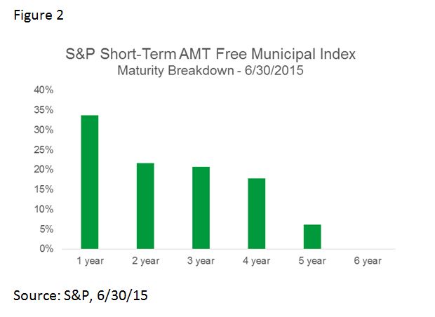
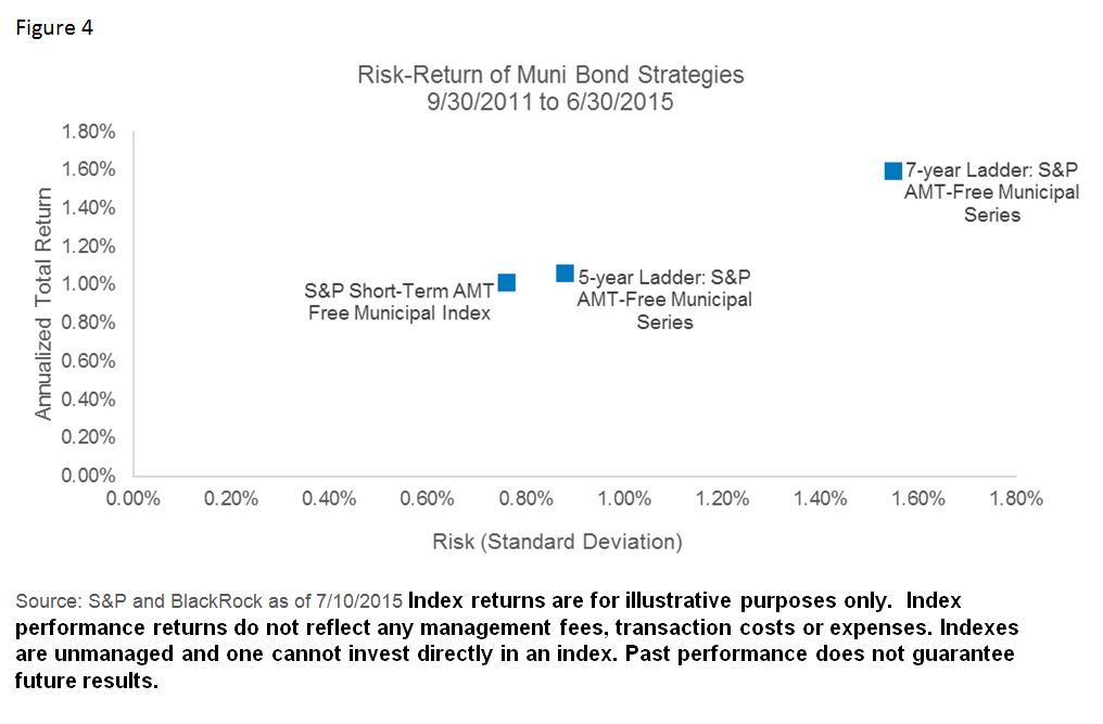
Let’s say an investor was considering three options: creating a five-year ladder, creating a seven-year ladder, or investing in a short-term municipal bond fund. For each of these investment options the investor is considering only non-callable, investment grade bonds. The performance of S&P AMT-Free Municipal indices can be used to measure how different segments of the muni market have performed over time; through them we can measure the historical performance of the three options. For our performance period we will look at September 2011 to June 2015. The S&P AMT-Free Municipal Series Indices include bonds that mature in each calendar year of the index name, and are available in maturities ranging from 2012 to 2023. A five-year ladder can be constructed using Municipal Series Indices that mature between 2012 and 2019. A seven-year ladder can be constructed using Municipal Series Indices that mature between 2012 and 2021. This analysis assumes that the investor is rolling the proceeds of each maturing index into a new longest rung on the ladder.

The performance of these ladder portfolios can be compared to the S&P Short-Term National AMT-Free Municipal Bond Index, which holds bonds from 0-5 years to maturity and rebalances monthly. The Short-Term index can be a good proxy for a short-term muni strategy that does not mature like a ladder.  The index is market cap weighted, and does not hold an equal weighted amount in each maturity year like the laddered solutions do.

The duration of the laddered strategies rolls down and then increases when an index matures and the proceeds are reinvested in the next rung. This is in contrast to the Short-Term index whose duration is more stable through time.

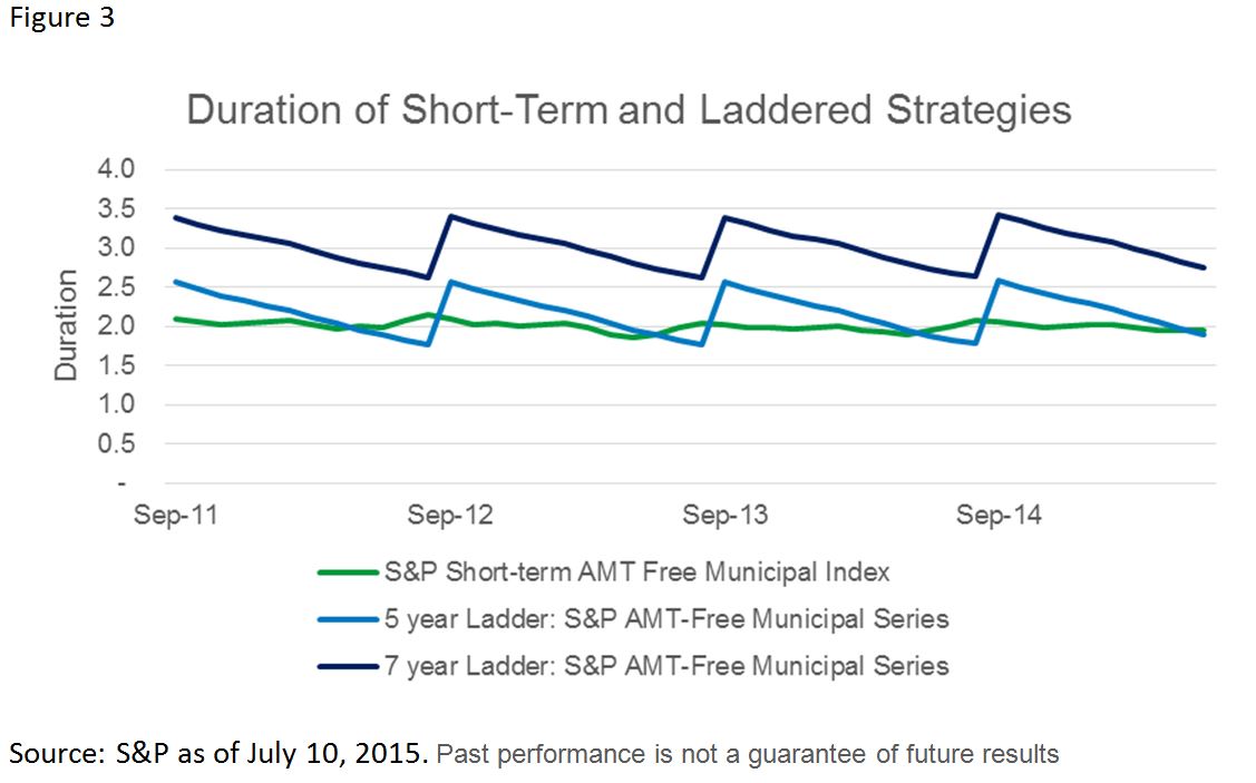
The performance of the 5-year ladder and the short-term index were similar. Note that the 5-year ladder had slightly higher return and volatility due to having an average duration that was slightly higher. Overall the duration differences between the three different portfolios was the largest driver of their performance differences.

Laddering a bond portfolio can provide investors with the flexibility to navigate the next round of rate hikes, while still helping meet their investment objectives. A laddering strategy can also provide more control over the portfolio, as an investor has an opportunity each year to reduce the size of the investor’s bond investment.  A short-term municipal bond strategy has provided a similar risk and return experience to the ladder options, and might be appropriate if the investor does not want to manage the maintenance of a ladder, or does not need the option of withdrawing proceeds from the investment on a regular basis.

—————————————————————————————————————-

The strategies discussed are strictly for illustrative and educational purposes and should not be construed as a recommendation to purchase or sell, or an offer to sell or a solicitation of an offer to buy any security. There is no guarantee that any strategies discussed will be effective.

Fixed income risks include interest-rate and credit risk. Typically, when interest rates rise, there is a corresponding decline in bond values. Credit risk refers to the possibility that the bond issuer will not be able to make principal and interest payments. There may be less information on the financial condition of municipal issuers than for public corporations. The market for municipal bonds may be less liquid than for taxable bonds. Some investors may be subject to federal or state income taxes or the Alternative Minimum Tax (AMT). Capital gains distributions, if any, are taxable.

iSHARES and BLACKROCK are registered trademarks of BlackRock, Inc., or its subsidiaries. All other marks are the property of their respective owners. iS-16101-0715

China’s actions in recent days to shore up its market are reminiscent of actions taken in the US after the 1987 stock market crash. Changes in monetary policy, support for margin calls and stock buybacks were all tried in 1987.  At the same time, some other steps taken in China currently – restricting short selling and halting stocks – were avoided.

The charts give show the run-ups and subsequent drops in both markets.  The first chart shows the CSI 300, the principal large cap index in China over the 12 months ended with July 21, 2015. Its run up from a year ago to its June 8^th peak is 90%; its subsequent drop is 22%, almost the same as fall in The Dow® on October 19, 1987. Of course, we don’t know whether China’s market has found a bottom yet.  The second chart shows the S&P 500® and The Dow for the full year 1987.

China’s central bank cut rates to support the market. The day after the 1987 crash the US Fed announced, “The Federal Reserve, consistent with its responsibilities as the Nation’s central bank, affirmed today its readiness to serve as a source of liquidity to support the economic and financial system.”  Sounds a bit like recent news from China.  The Fed followed its statement with reductions in the Fed funds rate and an overall move to easier money despite worries about the dollar and inflation at that time.  Commentators have noted China’s support for margin lending by providing funds. In 1987 the Fed banks in New York and Chicago stepped in and encouraged major banks to extend additional credit to investors facing margin calls.   In China pensions funds are being encouraged to increase their stock purchases.   While the extent of additional pension fund activity in 1987 isn’t known, stock buy backs by major corporations in the S&P 500 doubled from the pace experienced in January through September 1987.

Other Chinese initiatives do not mirror 1987 efforts in the US.  China has restricted short selling, halted trading in many stocks and prohibited IPOs.  The IPO action may not matter much since companies might not choose to do an IPO in the midst of market turmoil.  Restricting short sales appears to remove a key source of downward pressure in a market. However, without access to shorting, hedging is much more difficult; restricting short sales can actually be a deterrent to purchasers.  When investing in the BRIC (Brazil, Russia, India and China) countries first became popular,  S&P DJI introduced an unusual BRIC index which only includes stocks listed and traded in New York, London or Hong Kong – three markets where shorting is permitted.  This index’s success demonstrated the importance of access to short selling.

Halting stocks may be another attractive way to break a market’s fall. The US introduced circuit breakers – mandatory market time outs if major indices fall too far and too fast – after the 1987 crash. The challenge for either circuit breakers or wide-spread trading halts is how to restart the market.  As long as there is no trading, prices don’t fall. But, investors’ estimates of what the prices should be may still collapse, setting the stage for further declines when trading resumes.

With the final numbers for the second quarter of 2015 now available, the research firm ETFGI today brought some long-anticipated news: the size of the exchange traded funds market has finally exceeded that of its older, more well-to-do cousins.  It may have taken a little longer than we expected, but ETFs are now a bigger part of the market than hedge funds.

In order to explain why hedge funds might be losing out in the race for assets, we thought we would re-examine the challenge of replicating hedge fund performance.  When it comes to individual hedge funds, which are typically unconstrained by assets, leverage or geography, replication is a difficult objective.  When it comes to a broad hedge fund portfolio, replicating performance is easier than you might think.

To begin the replication process, our “hedge fund” is going to invest half its money in U.S. bonds, and the remainder in global equities.  (We’ll use the S&P U.S. Aggregate Bond index to represent the first portion and the S&P Global 1200 for the second.)  Assuming we also rebalanced on a monthly basis, here’s how our hedge fund would have performed over the past five years.  For purposes of comparison, we also show research firm HFR’s benchmark of hedge fund performance.  The HFR Fund-Weighted Composite Index includes funds which are no longer open to new investors, so it is a fair representation of what only the largest and best-connected asset owners may have available to choose from:

                    Sources: S&P Dow Jones Indices, HFR as of 30th June, 2015.

The pattern of returns seems similar, which is encouraging.  And our decision to allocate to equities and bonds in equal proportions means that the overall return from our replication strategy is much higher.  Well done us!

But congratulations are premature.  Our replication strategy does not include costs, or fees.  The replication costs of broad-based, passive indices are de minimis, but we should not undervalue our unique insights (we are replicating a hedge fund, after all).  A fee of 1.50% per annum seems reasonable, and we’ll take 15% of any profits (provided we’re at least breaking even over the past 12 months). Here’s how our performance looks now:

                    Sources: S&P Dow Jones Indices, HFR as of 30th June, 2015.

That’s more like it; our replication strategy now performs very similarly to the average hedge fund.  And when it comes to the pattern of returns, are we replicating the hair-trigger market-timing and monthly swings of the masters of the universe? Yes, we are:

                    Sources: S&P Dow Jones Indices, HFR as of 30th June, 2015.

One conclusion to draw is that perhaps there is a market for a product offering a 50/50 split of U.S. bonds and global large-cap equities, at a highly remunerative cost structure.  The other conclusion, perhaps shared by those whose continued flight to low-cost index funds are making the headlines today, is that the average hedge fund looks like a fixed blend of cheap investments, at high cost.

In this post, we are going to look at how April 2015 has fared compared with historical April months for the S&P/Case-Shiller U.S. National Home Price Index. Exhibit 1 depicts the historical monthly returns (April over March) of the S&P/Case-Shiller U.S. National Home Price Index, since 1987. All returns refer to April over March returns unless otherwise specified.

The April 2015 gain of 1.06% was the smallest April-over-March gain since 2011 (0.99%), but it was the largest monthly gain in the recent 12-month period ending April2015.

It can be seen from Exhibit 1 that the trough was around the 2008-2009 period. There also appears to be two peaks in the index—one in 2005 and a post-trough peak in 2013. The period between 1987 and 2003 appears to show moderate gains and losses, while the period from 2004 to 2015 seems more turbulent.

Exhibit 2 summarizes the peak and trough periods for all 20 metro areas in the S&P/Case-Shiller Home Price Indices and the S&P/Case-Shiller U.S. National Home Price Index. The first peak period is defined between year 2000 and the trough period of the S&P/Case-Shiller U.S. National Home Price Index in 2008.

Of the 20 metro areas, 12 peaked between 2003 and 2006. Atlanta, Chicago, Minneapolis, and San Francisco peaked as early as 2000, while Cleveland and Dallas do not appear to have had that first rally. Las Vegas had the biggest gain, at 5.4%, and Detroit had the smallest, with 0.9%. For the “second peak,” 15 of the 20 cities peaked in 2013, with Boston peaking as late as 2014, at 3.0%. The largest second peak was in April 2013 for San Fransisco , at 4.9%.

In terms of a trough, most of the cities had their largest April declines in 2008 and 2009. Chicago and Cleveland recorded their April troughs in 2007, while Boston and Dallas reported theirs in 2011. The largest April decline was in Miami in 2008, down 4.1%.

The S&P/Case-Shiller U.S. National Home Price Index (the “Index”) was launched on May 18, 2006. However, it should be noted that the historic calculations of an Economic Index may change from month to month based on revisions to the underlying economic data used in the calculation of the index. Complete index methodology details are available at www.spdji.com. It is not possible to invest directly in an index.

Now that negotiators have reached a deal aimed at reining in Iran’s nuclear program, Iran may get relief from some sanctions that may allow it to raise oil output. Though it could take time for supply to come onto the market, it depends on how long it takes for the International Atomic Energy Agency (IAEA) to verify all necessary nuclear-related actions have been met. Also, while oil in floating storage could come to market quickly (roughly 180 kb/d for 6 months according to IEA) and oil from already developed fields might be easier to deliver, underinvestment in production capacity and further negotiations of foreign investment from global oil companies may delay additional supply for significant time. It is extremely difficult to estimate future Iranian output not only from their own variables but based on how other suppliers will react to the news to maintain their market share ahead of Iran’s return.

The magnitude and direction of oil after Iranian supply comes to market is unknown. When less is known, volatility generally picks up as has happened in past oil crises. Also historically, open interest has had to crash before oil stabilized. Not only may OPEC’s last decision to continue production backfire from fund managers cutting their bets, but recent trade data from the Commodity Futures Trading Commission (CFTC) shows speculators have made their sharpest crude selloff in more than two and a half years. This is a critical point because the open interest is now at its lowest monthly peak in 2015. Also, the open interest has historically dropped about 1/3 before volatility normalized and now the numbers are showing the drop from roughly 500,000 to 300,000. This may be an inflection point indicating market rebalancing may be in its early stages.

Although the open interest may be collapsing now to initiate the start of the bottoming process, there is trouble for Iran. The timing is terrible because oil has continued to be supplied in excess (as shown below by the negative roll yields from contango) since July 2014. As they re-enter the market, it may cause more downward pressure on oil prices, limiting the upside on their revenue.

A consequence of Iran’s lower potential revenue is that it may hinder its ability to import healthy food to feed its population. Since its climate is not ideal for production, and is warming, Iran is food insecure and needs to rely heavily on imports. Iran imported $214 million worth of wheat in 2013 with other major imports including corn, soybeans and meat but malnutrition and obesity has risen as imports of cheaper sugar (DJCI Sugar lost 14.1% YTD as of July 13, 2015) have replaced many fruits and vegetables.

The concurrent glut of oil as Iran re-enters the market with the agricultural and livestock term structures that are now showing shortages can work against the budget both ways. This is particularly bad timing as contango (shown as negative) is now flipping towards backwardation (shown as positive) in these commodities – with the exception of soybeans:

Even worse for Iran is that importing food may be more expensive than ever due to the highly predicted El Niño. Agricultural prices have been increasing at an accelerated pace with each El Niño since 1982 by roughly 2.6% with large possible spikes following the heat waves.