Indexology^® Blog

The Narendra Modi government will soon complete its five years in power. With polling underway to elect the next government, India is in election mode. Everyone is discussing politics and predicting the election results. The backers of the current government claim that the return of Modi will provide stability and ensure development. On the other hand, those backing the opposition, the Congress-led United Progressive Alliance, claim that a change in government is required in order to maintain secular harmony in the country. Neither side would welcome a hung parliament.

Over the past five years, the government made several landmark policy decisions and initiatives like the Goods and Services Tax (GST), demonetization, Insolvency and Bankruptcy Code, and Real Estate (Regulation and Development) Act, among others. Many of the reforms have had a major impact on the Indian economy. Even after disruptive reforms like the demonetization and GST, economic growth is back on track. Opinion surveys conducted before the polling suggest a close fight and the current government may not achieve the majority it got last time. The outcome is anyone’s guess until the counting begins on May 23, 2019.

The S&P BSE SENSEX TR moved from 30,242.22 on April 30, 2014, to 56,443.02 on April 30, 2019—a five-year absolute return of 86.64%. The S&P BSE AllCap, a broad benchmark index with over 1,000 constituents, had a five-year absolute return of 94.49%. Among the size indices, the five-year absolute return of the S&P BSE MidCap was the highest, at 115.35%, followed by the S&P BSE SmallCap, at 103.98%, while the S&P BSE LargeCap was at 86.70%. Exhibit 1 depicts the total returns of the S&P BSE SENSEX, S&P BSE AllCap, S&P BSE LargeCap, S&P BSE MidCap, and S&P BSE SmallCap for the five-year period ending on April 30, 2019. The capital markets in India have presented significant returns to investors in the past five years.

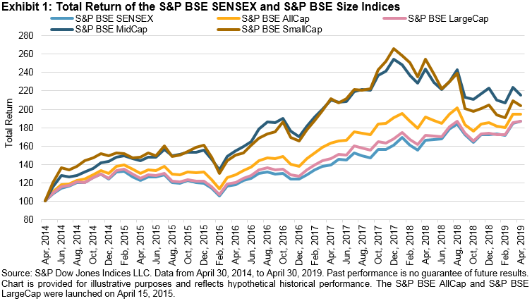
Exhibit 2 provides the five-year absolute returns of the S&P BSE AllCap Series. Among the sub-sector indices in the S&P BSE AllCap, the S&P BSE Finance and the S&P BSE Energy posted the best five-year absolute returns of 133.40% and 130.81%, respectively, while the S&P BSE Telecom had the worst return, at -15.92%.

Source: S&P Dow Jones Indices LLC. Data from April 30, 2014, to April 30, 2019. Past performance is no guarantee of future results. Table is provided for illustrative purposes and reflects hypothetical historical performance. The S&P BSE AllCap, S&P BSE LargeCap, S&P BSE Finance, S&P BSE Energy, S&P BSE Consumer Discretionary Goods & Services, S&P BSE Basic Materials, S&P BSE Utilities, S&P BSE Industrials, and S&P BSE Telecom were launched on April 15, 2015.

Market gains in the first four months in 2019 more than made up for what it lost in the turbulent last quarter of 2018 as the S&P 500 jumped 18%. Predictably enough, the S&P 500 Low Volatility Index^® trailed the broader benchmark (up a “mere” 16% in the first four months), although Low Vol has led the broader benchmark during May’s pullback.

The May rebalance (effective at the close on May 17^th) yielded minimal change in the sector distribution within the low volatility index. The most significant changes include added allocations to Financials and a scaling back of Technology.

Financials Became More Significant as Health Care and Technology Scaled Back in the Latest Rebalance for the S&P 500 Low Volatility Index

Trailing one-year volatility for each S&P 500 sector declined in the last three months. The volatility reduction was more or less equally distributed, so it’s not surprising that the latest rebalance wrought minimal changes in sector exposure for Low Vol. In fact, this latest rebalance is notable for its low turnover. The index replaced only 9 names, nearly half the count of the average of 17 over the last two years.

252-Day Volatility Declined Across All S&P 500 Sectors Compared to Three Months Ago

Global equities have been turbulent recently as a combination of stalled trade negotiations and announcements of tit-for-tat tariffs increased the prospect of a trade war between the U.S. and China.  After its historic start to the year, the S&P 500 is down 3.7% so far in May, while many other markets have also faltered month-to-date.  Amid the recent market jitters, many investors may be interested in strategies that help navigate periods of heightened volatility.

Many index-based strategies are designed to ride out turbulent times.  Among the most popular defensive equity strategies are low volatility and minimum volatility indices.  However, while both strategies are based on the low volatility anomaly and have similar names and objectives, they are constructed differently.  Low volatility indices rank constituents by their trailing volatility and select the least volatile stocks, whereas minimum volatility indices use an optimization-based approach to construct the least volatile portfolio.  Hence, low volatility indices comprise only low volatility stocks, whereas minimum volatility indices may contain highly volatile stocks.  Exhibit 1 shows the differences in portfolio construction for the S&P 500 Low Volatility Index and the S&P 500 Minimum Volatility Index.

Exhibit 1: Low & Minimum Volatility Indices are constructed differentlySource:  “Inside Low Volatility Indices”.  Table is provided for illustrative purposes.

Exhibit 2 shows that the differences in methodologies impacted the indices’ risk/return profiles: the S&P 500 Low Volatility has offered greater downside protection – and higher risk-adjusted returns – than its minimum volatility counterpart since December 1990.  Indeed, the low volatility index typically captured less than half of S&P 500’s total return in “down” months (determined by whether the S&P 500 posted a monthly decline), compared to around 70% for the minimum volatility index.

Exhibit 2: Low & Minimum Volatility Indices Behaved Differently

Another difference between low and minimum volatility indices is their geographic revenue exposure: around 80% of the S&P 500 Low Volatility’s revenues come from the U.S, compared to 66% for the S&P 500 Minimum Volatility.  Exhibit 3 helps to explain this result; it shows the sector exposures (height of the bars) and the domestic revenue exposures (bar labels) of companies within each sector for each index.  Clearly, the low volatility index has sizable allocations to more domestically-focused companies, especially within the Utilities, Real Estate, and Financials sectors.  On the other hand, the S&P 500 Minimum Volatility has greater exposure to companies that are more reliant on revenues from abroad.

Exhibit 3:  Low & Minimum Volatility indices may have different revenue exposures

As a result, while low and minimum volatility strategies have similar sounding names and objectives, they can behave differently over time.  Combined with differences in sectoral allocations and geographic revenue exposures, and how this may impact performance in the event of an escalation of trade tensions, market participants may be well served to take a deeper look inside low volatility indices.

Economics used to be Political Economy. Today politics in encouraging economics to look at different ideas such as Modern Monetary Theory. MMT argues that a country which borrows in its own currency will never default: as long as the US sells bonds denominated in US dollars, it won’t matter how big the federal budget deficit becomes.

MMT isn’t a free pass to unlimited government spending. However, it makes a case that a new government program doesn’t need to be matched by tax increases or spending cuts. Medicare and defense spending are not about to bankrupt the government. Under MMT, tax policy as well as monetary policy would be used to control inflation.

1. If a government borrows in its own currency it can always avoid default by printing more money,
2. Inflation can be controlled through higher taxes to limit spending,
3. Monetary policy can focus on interest rates rather than inflation and growth,
4. Fiscal policy is freer to support economic growth and jobs.

The U.S. normally borrows in its own currency – the Treasury sells bills, notes and bonds denominated in U.S. dollars. The Federal Reserve buys treasuries by crediting a bank’s account at the Fed – it prints money — to pay for treasuries. As long as the Treasury keeps issuing debt, the Fed can keep creating bank reserves and buying bonds. Therefore, the government cannot default as long if its debts are in dollars. If investors lose faith in US treasuries and decide to buy corporate or foreign bonds, the Fed could still keep printing money and funding the government. As extreme as this may sound, it is not that different from Quantitative Easing (QE). Under QE, the Fed bought bonds by crediting banks’ accounts at the Fed in an effort to increase spending across the economy and raise economic activity.

Of course, excessive borrowing and unlimited printed money is not a good approach to government finance. There aren’t any free lunches in economics. Were the government to spend without limit it would boost the demand goods and services, push prices up, squeeze resources and accelerate inflation. Under a traditional approach to inflation control via monetary policy, the Fed would raise interest rates, to curtail economic activity and cut inflation. Under an MMT monetary regime, the Fed would be committed to funding the treasury. Inflation would be controlled through higher taxes. If large increases in the government or the private sector spending caused inflation, the higher taxes would lower private sector spending while cutting the amount of government debt the Fed needed to buy.

Today the federal budget deficit is 4%, and total federal spending is 21%, of GDP. The 4% is funded by selling debt; the rest (17%) is paid for by federal tax revenues. Switching to MMT would disrupt the economy and create a flood of debt and cash. If taxes were trimmed, private sector spending would balloon and drive inflation sky high.

While few analysts looking at MMT would suggest abandoning the current monetary policy structure, many believe that government-spending decisions should not be dominated by fears of larger deficits. Spending proposals should be evaluated on their benefits and costs, not by what program must be cut to pay them. Behind every government program there is a Congressman, Senator or cabinet secretary who will fight to keep – or raise – its budget. As long as each new dollar must be paid for by giving up an old dollar, there will be very few new dollars even if the return would be substantial.

Although MMT is a new angle in deficit debates, the federal deficit is as old as the country. As the chart shows, deficits have been the rule in this century and more often than not over the last 90 years.  The message to take from MMT is that a bit more federal spending will not bankrupt the country whether or not monetary policy is turned on its head.

The S&P 500^® was up 3.93% in April, marking the fourth consecutive month of gains. The YTD gain of 17.51% was the best since 1987 and the fifth-best in the entire history of the index. The index set a new all-time high in April, surpassing the previous high close from Sept. 20, 2018. This completed a full recovery from the 19.86% decline in the fourth quarter of 2018. Over the past 30 years, the first four months were all consecutively positive six other times, averaging YTD returns of 10.59%. Notably, all six instances ended the respective year higher than the April-end level, with an average annual return of 25.10% (see Exhibit 1).

Both the S&P MidCap 400^® (18.5%) and SmallCap 600^® (15.4%) have had their best-ever start to the year through the end of April. Both mid and small caps were positive in April, rebounding after both were negative in March. Of the 11 sectors, 8 were positive in both the large- and mid-cap segments. Of the small-cap sectors, nine were positive. Financials was a top-performing sector, with the S&P 500 Financials the best at 8.84%. Health Care, Energy, and Real Estate were the bottom three sectors. The largest spread between size segments was within the Communication Services sector, with the large cap gaining 6.22% and small cap losing 2.15%. Additionally, value outperformed growth in all three size segments. Overall, 29 of the 42 segments of the U.S. equity market had higher returns in April compared with March, and only eight were negative.

Considering the historic YTD gains as the month of May begins, the common “Sell in May and Go Away” adage comes back into focus. Despite being somewhat of an investing axiom, it is a recurring debate. The over 90-year history of the S&P 500 can be used to evaluate historic results for the November through April and May through October periods. Overall, the S&P 500 averaged a 1.98% return in the May through October periods and was positive in 59 of the 90 periods.

Performance has tended to be lower in the May through October periods. Over the 90 years since Oct. 31, 1928, the S&P 500 on average returned 3.25% less in the May through October period compared with the preceding November through April period. The performance on average was lower, but there were 29 instances that the May through October period return was higher than the preceding November through April, including 15 instances that the November through April period was negative and May through October was positive. This compares to 21 instances when the November through April period was positive and the following May through October period was negative. Regardless of which was higher, there were 43 instances that both the November through April and following May through October periods were positive, and 11 instances that observed negative returns in both periods.

Throughout the ongoing bull market, the November through April period has outperformed the following May through October period by an average of 6.28%. The May through October period outperformed the prior November through April period only once (2016) and was negative three times (2010: -0.29%; 2011: -8.09%; 2015: -0.30%). However, the average return for the May through October periods remained positive, at 2.53%.