Indexology^® Blog

With 2017 in the rear view mirror, we can look back and observe that short VIX strategies rank as one of the most profitable strategies of the year. The S&P 500^® VIX Short-Term Futures Inverse Daily Index returned 186.39%, and selling VIX futures has become a popular income-generating strategy. 2017 was also a year marked by an extraordinary level of low volatility. VIX has been hovering around 10 and dipped below 10 more than 50 times; on Nov. 3, 2017, VIX posted its all-time low   of 9.14.

Contrary to the traditional “buy low, sell high” investing principle, in VIX trading, low volatility encourages more selling, rather than buying, on VIX futures, which is counterintuitive given the often-discussed, mean-reverting property of VIX.

There are two factors market participants need to consider when confronting this mystery.

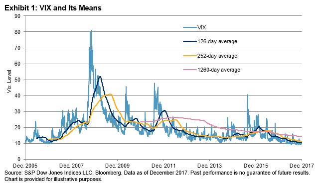
First of all, VIX displays local mean reversion. That is, it tends to return to its short-term local mean, rather than to its long-time average. Exhibit 1 shows VIX numbers, with 126-, 252-, and 1,260-trading-day averages. We can see regime shifts of VIX over its history. The long-term mean (in this case, five-year average) has very little indicative power on the current VIX level. As VIX tends to rise much faster than it falls, in low VIX markets, such as in 2013, 2014, and 2017, the spot may remain below its long-term mean for extended periods.

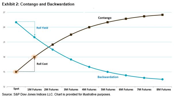
Second, we need to understand that VIX futures indices and their index-linked investment vehicles provide short exposure to VIX futures, not the spot. A key concept for any futures contracts, not just VIX futures, is the futures term structure, since the futures curve shape dictates whether rolling futures over time incurs cost or benefit. Futures are in contango when the futures term structure is upward sloping, meaning the futures prices are more expensive than the spot. Futures are in backwardation when the futures term structure is downward sloping, meaning the futures prices are less expensive than the spot (see Exhibit 2).

Although the VIX spot is somewhat mean reverting, holding a long position in VIX futures over the long term tends to produce losses, because the VIX futures term structure is usually in contango, as market participants generally associate more uncertainty with longer time horizons. However, in a stressed market where immediate risk is perceived by most market participants, the VIX futures curve tends to flip into backwardation.

To highlight, we can use the widely followed S&P 500 VIX Short-Term Futures Index as an example. It rolls continuously from the first-month futures to the second month. Exhibit 3 shows the price difference of these two contracts starting on Jan. 3, 2005, calculated as the second-month VIX futures price minus the first-month VIX futures price. Among these 3,272 trading days, contango occurred on 2,718 days (83%) between the first- and second-month VIX futures. Given that approximately 5% of the portfolio is rolled on a daily basis, the average daily roll cost is 29 bps.

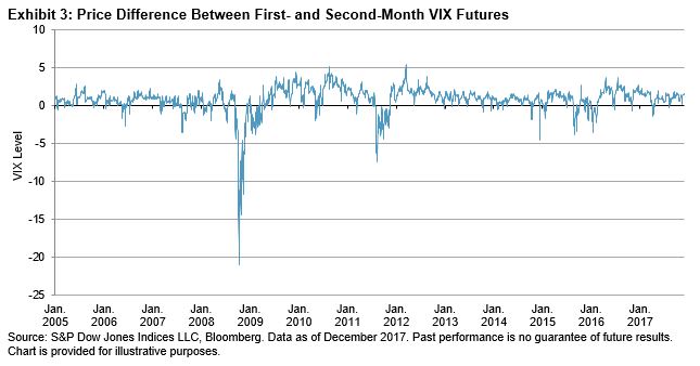
This roll cost may seem minor on a standalone basis, but its cumulative impact on VIX futures performance is significant. If VIX remains unchanged for a year, the index can potentially lose about half of its value in the continuous daily roll process.

Therefore, we need to take into account that VIX spot tends to revert to its short-term mean, and the current low volatility environment may persist until a regime shift. When VIX is low and the market is calm, the VIX futures curve tends to be in contango, which encourages shorting VIX futures strategies, as we witnessed in 2017.

The first estimate of US GDP for the fourth quarter is set to be released this Friday and the median forecast is 3.0% according to MarketWatch, which if met or exceeded will be the first time 3 consecutive quarters to show at least 3% growth since the first quarter of 2005.  While this is supportive for the entire U.S. equity market, small-caps may gain most (except small-cap telecom.)

On average for every 1% of GDP growth, the small-cap index, S&P 600, historically gained 5.1%.  This is only slightly better than the mid-cap index, S&P 400, that gained on average 4.9% but is significantly better than the large-caps of the S&P 500 that rose just 4.0%.  Also notice growth and value styles dilute the impact of GDP growth on small cap, though significantly lift large-cap.

Technology mid-caps has been the big winner, gaining 7.4% for every 1% rise in GDP.  However, financials, health care and energy were most positively sensitive in small caps, rising on average 6.9%, 6.4% and 6.3%, respectively, for every 1% GDP growth.  Although only small-cap telecom lost on average with GDP growth, consumer discretionary, materials, technology and industrials did not rise as much as the composite S&P 600.  Therefore, even though the small-cap index is hard to beat, there are chances if GDP growth accelerates.

While the economy seems strong and the stock market is booming, the U.S. dollar is down about 3.3% so its impact should be addressed.  In the past 10 years, a falling dollar is better for stocks than a rising dollar, and mid-caps benefit most from the falling dollar.  On average for every 1% the dollar falls, mid caps rise 3.2%, small caps gain 3% and large caps gain 2.6%.  A rising dollar doesn’t hurt, but when the dollar rises stocks are less sensitive to the move.   However, not surprisingly, a rising dollar does hurt energy, the most negatively correlated sector to the dollar.  Oppositely, as the dollar weakens, energy, especially in small caps, may gain most.

More on the U.S. dollar’s stock market impact will be in another post soon, but in the meantime note large-caps do worst of the sizes with both GDP growth and a weaker dollar.

Latin America closed 2017 on a high note. This is the annual edition of this report where we will review the 2017 performance of country and regional indices, as well as the best performers and those that lagged behind.

Latin America’s annualized returns, as measured by the S&P Latin America BMI (the broad regional index) and the S&P Latin America 40 (the narrow, blue-chip index), have even surpassed the S&P 500 and the S&P Global 1200, which measures the 1,200 largest, most liquid companies from around the world. Latin American regional and country indices are now showing two consecutive years of positive double-digit returns, bringing their three-year returns into positive territory. There is still some ground to cover before the 5- and 10-year returns also move to the positive side, although the gap is closing.

Despite political challenges in Brazil, elections in Chile, natural disasters in Mexico, and extraordinary circumstances of corporate corruption that affected the entire region from top to bottom, all stock markets in the region fared exceptionally well in 2017, as reflected by their respective country indices: the S&P Brazil BMI, S&P Chile BMI, Mexico’s S&P/BMV IRT, S&P Colombia BMI, and S&P/BVL Peru General. In particular, the three largest markets had the biggest impact on regional returns. Brazil, which represents nearly 58% of the S&P Latin America BMI, had an annual return of 26.1%. Chile, the third-largest market in the region by weight, had an annual return of 45.2%. Mexico, the second-largest market in Latin America, representing nearly 24%, generated a strong return of 11% for the year. Argentina was the monster (in a good way) of the region. Because the market is classified as a frontier market and not emerging, it is not currently considered part of the S&P Latin America BMI; however, it merits mentioning that its performance for the year was outstanding, at 73.1% in USD and 106% in ARS.

So, what were the drivers? Based on historical data, Latin America was the last region to catch up with other global markets. Positive global investor sentiment, good corporate valuation, along with many other accommodative financial factors (such as low market volatility, as measured by VIX^®, low interest rates, low inflation) and rising commodity prices (such as gold and oil) contributed to the markets performing well in 2017. In Latin America, only 58 out of 285 companies in the S&P Latin America BMI had negative one-year price returns. This means that 85% of the companies in the index yielded positive returns. As of year-end 2017, the top 28 stocks, representing 50% of the index, had an average annual return of nearly 36%.

Economic growth has picked up in Latin America based on Q3 2017 data. GDP for the region has expanded at a stronger rate since Q1 2014,[1] leaving the previous year’s recession in the past. While analysts expect the economies to continue to grow, there is some hesitation on these projections, given the major elections coming up for Brazil, Colombia, and Mexico. New administrations can either help or hinder the necessary economic policies to continue the region’s expansion. While they seem confident, market participants are taking a moment to see what the approach will be for 2018. This certainly will be an interesting year for the region.

To see more details about performance in Latin America, please see: S&P Latin America Equity Indices Quantitative Analysis Q4 2017.

[1] Focus Economics, “Economic Snapshot for Latin America,” www.focus-economics.com/regions/latin-america. Dec. 7, 2017.

The three pillars of conventional retirement income are social security retirement benefits, pensions from employment, and personal savings. There are, however, other potential sources of retirement income that are not mentioned often enough. These include (a) the cash value of one’s whole life insurance policy, (b) the home equity value of one’s residence, and (c) the pre-funded nature of the long-term care insurance policy.

Let’s dig a bit deeper into the nontraditional sources noted above.

(a) The premium for a whole life insurance policy is generally much higher than that of a term life insurance policy. Hence many tend to shy away from purchasing the whole life insurance. However, the premium paid for a whole life policy can be viewed as consisting of a premium for an equivalent term life policy plus a contribution to an investment account maintained for the insured by the insurance company. The balance in this investment account is known as the cash value of the whole life insurance policy. As time passes, if one is still alive, this cash value will also grow, due to the fact that new premiums are adding to the account balance and the entire balance is increasing at a rate tied to the performance of the insurance company’s general account.

When the insured individual gets older, say age 75, if the objective of protection is no longer an issue, the insured has the option to surrender his policy and tap into the cash value as a source of income.

(b) The home equity value of one’s residence can also be accessed by using the property as collateral for either a home equity loan or a reverse mortgage. The advantage of this type of secured borrowing is that one can continue to stay in one’s residence without resorting to a sale.

(c) The last source, the long-term care insurance policy, is intended to provide funding for healthcare-related expenses, which can be expected to be ever-present in old age. A long-term care policy, purchased when one is younger, behaves as if it’s prefunding one’s late-life healthcare expenses on a level-payment basis. In this way, even though it is a non-cash source of income, since it takes care of the healthcare-related expenses when they’re incurred, it can be thought of as a cash item. Typically, for the long-term care policy to be activated, a doctor’s approval is required by the insurance company, and the insurance company would reimburse the healthcare providers directly.

For one to feel secure in retirement, monthly cash incomes are needed to take care of both the core expenses and discretionary ones (such as for travel and entertainment). What has often been overlooked are the benefits from the unconventional sources, both as additional sources of cash (for example, from one’s cash value account or home equity loans) or as indirect non-cash contributions (such as the expenses covered by one’s long-term insurance). These additional sources of support need to be taken into account in one’s financial life planning as well.

Most sentient investors are aware of the low volatility that characterizes the current environment, with the S&P 500^®’s trailing twelve-month annualized volatility at approximately half its level from a year ago. This trend was driven in part by some significant negative inter-sectoral correlations, for example between information technology and real estate versus financials, and energy versus information technology (see Exhibit 1).

Going a step further at the sector level, we observe decreases in volatility across the majority of sectors. Most notably, energy had the largest decrease (see Exhibit 2).

As illustrated in the most recent sector dashboard, the S&P 500 Energy sector’s trailing twelve-month annualized volatility was 13.2% as of Dec. 29, 2017—approximately half the sector’s 23.6% volatility from the prior year, with volatility declining steadily over the past twelve months. Historically, energy volatility has ranked roughly at the median of all sectors. We witnessed an aberration in recent years, as the sector’s volatility reached peak levels. However, this trend has reverted during the past year.

Market volatility can be understood in terms of two components: dispersion and correlation. Dispersion measures the degree to which index constituents perform differently, and correlation measures the tendency of index constituents to rise or fall at the same time. The decline in energy sector volatility has been driven by declines in both correlation and dispersion.

Exhibit 3 shows that the average trailing twelve month dispersion for the S&P 500 Energy sector was 13.4% as of Dec. 29, 2017, versus 20.5% one year prior. Similarly, the average trailing twelve month correlation for the S&P 500 Energy sector was 0.43, versus 0.57 one year before.

While energy was the second-worst-performing sector in 2017, performance has picked up so far in 2018, with the sector up 5.9% for the month as of Jan. 19, 2018, aided by strengthening oil prices. Will this performance tailwind reverse last year’s decline in volatility? We shall wait and see.