Indexology^® Blog

Factor Definition
The fixed income investment community has long used volatility in analyzing bond valuations and identifying investment opportunities.  We have defined volatility as the standard deviation of bond yield changes for the trailing six-month period.  All else being equal, the more volatile the bond yield is, the higher the yield needs to be in order to compensate for the volatility risk.

For the credit spread factor, we consider the option adjusted spread (OAS), which represents the yield compensation for bearing credit risk, as well as other risks associated with credit.  OAS is a common measure of valuation for corporate bonds.

Factor Identification
To identify the factors that could enhance security selection, we computed the performance statistics of the quintile portfolios ranked by each factor and demonstrated the strong relationship of factor exposure, portfolio return, and return volatility.

The underlying universe for our study was the S&P U.S. Issued Investment Grade Corporate Bond Index (U.S. issuers).  The index seeks to measure the performance of investment-grade corporate bonds issued by U.S.-domiciled corporations denominated in U.S. dollars.  Based on the availability of the constituent data and the yield curve, the period covered in the study was from June 30, 2006, through Aug. 31, 2015.  We derived an investable sub-universe (details in next blog) based on the broad universe and constructed quintile portfolios of the investable sub-universe.

To form the quintile portfolios, we first ranked bonds within the investable sub-universe by each factor (credit spread and low volatility) and divided the universe into five groups, with higher values ranking higher (Quintile 1) for credit spread and lower values ranking higher (Quintile 1) for low volatility.  It should be noted that these two single-factor portfolios did not control for either duration or credit rating.  Exhibit 1 shows the performance statistics of ranked quintile portfolios by single factors.

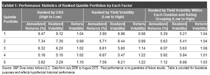
Exhibit 1 confirms a positive relationship between credit spread, portfolio return, and return volatility; i.e., the wider the credit spread is, the higher the return and return volatility are (Quintile 1).  Contrary to the credit spread factor, we observed a non-linear relationship between risk and return for the low volatility factor.  The Quintile 1 portfolio, containing the least volatile bonds, had the lowest return and the highest level of realized portfolio volatility.

Exhibit 1 also includes performance statistics for the quintile portfolios formed by ranking the low volatility factor within each duration and rating grouping.  These modified quintile portfolios displayed a generally positive relationship between the low volatility factor, return, and return volatility, as expected.

This demonstrates that applying the low volatility factor without taking duration and quality into consideration is not consistent in explaining portfolio return and risk.  This is because simply ranking bonds by yield volatility across the universe can potentially result in highly concentrated portfolios in duration or quality, which in turn can cause greater portfolio volatility.  This can be particularly exacerbated when long-duration bonds exhibit lower yield volatility than short-duration bonds when the market is quiet.

These findings confirm that credit spread and low volatility factors can effectively explain portfolio return and volatility and present the necessity of applying factors while taking duration and quality into consideration.

Despite the fact that many single-factor strategies have empirically delivered positive excess returns in the long run, they have suffered periods of substantial underperformance under certain market conditions due to their cyclicality.  Blending a number of desired factors with low correlations is a potential way to attain more balanced and diversified portfolios.  The obvious questions that arise are: Are they likely to achieve better performance?  How do they behave in different financial environments?

Our stylized portfolios that blend six factors (volatility, value, quality, size, momentum, and dividend yield) with four different strategies (marginal risk contribution, minimum variance, Sharpe-ratio weighted, and equity weighted) demonstrated higher risk-adjusted returns than the S&P 500^®, with a lower tracking error than most single-factor strategies (see Exhibit 1).

Over the entire period, marginal risk contribution and equal-weighted strategies exhibited less cyclicality than other multi-factor and most single-factor strategies.  They achieved more consistent and higher excess return than other strategies across various market cycle phases.  On average, they produced higher information ratios and a higher incidence of outperformance during recovery and bearish periods.

The minimum-variance strategy had a significantly lower information ratio and a lower incidence of outperformance in bullish and recovery markets, similar to, but less defensive than, the single low-volatility strategy.  The Sharpe-ratio-weighted strategy performed well in bear markets, but it significantly lagged the S&P 500 in recovery periods.  This suggests that using recent momentum to tilt factor exposures did not improve the risk-adjusted return of the multi-factor portfolio, even though it had a lower drawdown as a result of the strategy moving into cash during the global financial crisis.

For more information on our research on multi-factor smart beta strategies, please click here, where you will also find details about:

• What is driving risk/return of various smart beta strategies, and
• How each of the smart beta strategies have performed in different macroeconomic and market environments.

Factor-based investing in equities is a well-established concept supported by over four decades of research. However, factor-based investing in fixed income remains in its nascent stages. Our analysis has found that factor-based fixed income strategies implemented in a rules-based, transparent index can represent an alternative tool for fixed income portfolio construction. In the next few blogs, we will detail our approach to and back-tested results of employing credit spread (value) and volatility as factors in order to systematically construct a portfolio of U.S. investment-grade corporate bonds.

Investment Philosophy
In practice, an active portfolio manager for a corporate bond mandate mostly focuses on credit returns, specializing in expressing views on the direction of credit spreads and security selection. We propose a two-factor model to seek to collect an active return from security selection, identifying relative value opportunity in credit returns while keeping portfolio duration and credit duration natural to the underlying universe.

Two Factors: Volatility and Credit Spread
To achieve better security selection, we chose two factors that empirically have demonstrated a strong relationship between factor exposure and performance statistics and that have long been incorporated in investment analysis by corporate bond portfolio managers. Our selection of factors was by no means exhaustive.

The fixed income investment community has long used volatility in analyzing bond valuations and identifying investment opportunities. We have defined volatility as the standard deviation of bond yield changes for the trailing six-month period. All else being equal, the more volatile the bond yield is, the higher the yield needs to be in order to compensate for the volatility risk.

For the credit spread factor, we consider the option-adjusted spread (OAS), which represents the yield compensation for bearing credit risk and other risks associated with credit. OAS is a common measure of valuation for corporate bonds.

Back-Testing Total Return

Exhibit 1 shows the cumulative total return for our two-factor model versus the broad market. In the next post, we will demonstrate how we identify these two factors.

One of the few things more reliable than active managers’ general run of underperformance is their confidence that, despite what happened last year, this year will be different.  Two years ago, e.g., active managers were arguably poised to excel because correlations had declined from their financial crisis peaks; a year ago it was active managers’ putative ability to navigate declining markets that provided the rationale.  The data contradict both arguments, of course — there’s no reliable tendency for active management performance to improve when correlations are low or when markets are weak.

When considering whether we’re in an attractive environment for active management — the long-sought “stock picker’s market” — it’s important to bear in mind the difference between the existence of skill and the value of skill.  Suppose I am blessed with the ability to identify stocks whose performance is one standard deviation better than a market index’s average return.  The value of my skill will increase as the spread among stocks in the index widens.  If I were (or thought I were) a good stock picker, I would want to operate in an environment of widely-dispersed returns.

Dispersion, in fact, is a systematic measure of the weighted standard deviation of index component returns, and gives us a way to gauge the potential benefit of active stock selection.  In January 2016, dispersion in the S&P 500 rose sharply, reaching its highest level in more than four years.

One month does not a new regime make, of course, but the trend in the data suggests that S&P 500 dispersion may be beginning to climb above its long-compressed level.  High dispersion goes hand in hand with high volatility, however, and high volatility often signals negative returns.

Thus the irony: active equity managers may finally have the stock picker’s market for which they’ve hoped.  But the price of a stock picker’s market may be, at least in the short run, a period of volatile and negatively-biased returns.

Considering commodities were on pace to set the worst January since 1975 at one point, down 14.3% by Jan. 20, the final monthly loss of just 5.2% is impressive. The S&P GSCI Total Return rebounded 10.6% with nine of the twenty four commodities posting gains for the month.

Does this mean commodities hit the bottom or that this is just a bounce in a much darker scenario? That probably depends on the oil supply decisions from Saudi Arabia, Russia and Iran, in addition to Chinese demand growth, the strength of the dollar and the weather. However, an examination of the historical annual performance of the S&P GSCI based on the direction of returns in January for single commodities and sectors gives hope that 2016 may be a positive year.

Again, nine of the twenty four commodities in the S&P GSCI were positive in January. Historically, there is a higher chance the year will end positively than negatively based on the first month’s performance for seven of those commodities. The most interesting statistic of the positive single commodities is that when gold has gained in January, the S&P GSCI has gained for the year almost 3 of every 4 times, or in 72% of the time. Gold gained 5.3% in January 2016, so there may be a 72% chance of a positive year in 2016 for the S&P GSCI, based on that historical data point.

What is more compelling is that of the fifteen negative commodities, only three have had the majority of years ending negatively based on their losing January months. For most of petroleum, the first month’s direction is only as good as a coin flip, but when Brent Crude loses, that has been a good thing in 63% of years for the S&P GSCI. Another namesake commodity, copper, that many watch as an indicator of economic health, lost 3.1% in January, but based on history, the S&P GSCI has gained in 68% of years where copper lost in the first month.

On average, there is a 59% chance of a positive year in 2016 for the S&P GSCI  based on the number of times in history positive years have followed the direction of commodities this past January. The sectors tell the same story with a slightly higher chance, 64%, of a positive commodity year in 2016. Still, the outcome for the year is uncertain, especially since the direction of the January performance of the S&P GSCI itself, doesn’t say much. According to the historical data, there is only a slightly greater chance, 53%, of a negative year than a positive one in 2016.